Nicolas Grimaldi, David Kaber, Ryan McKendrick, Yunmei Liu (2024). Deep Learning Forecast of Perceptual Load Using fNIRS Data. In: Human Factors in Design, Engineering, and Computing. AHFE Open Access, vol. 159, pp. 12–22. https://doi.org/10.54941/ahfe1005563
In this paper, we present a novel approach to forecasting perceptual load in demanding piloting tasks, based on neurophysiological response data. We introduce a forecasting framework using a multinomial classification model paired with deep learning sequence-to-sequence models. The study compared the performance of seven different deep learning models, including GRU, Transformer, and linear models with a 10s outlook against a statical model benchmark. For analysis and validation purposes, the dataset was first split into training and testing sets, and the training set was further used to perform a 5-fold cross validation. The cross-validation results were used to evaluate generalization in terms of the regression loss used to train the deep learning models, while the testing set was used to evaluate the classification performance, including macro and weighted recall, precision and F1 scores. The prediction time for each model (computational demand) was also analysed for insight into model viability for real-time perceptual load forecasting.
Perception, as addressed by Lavie (1995), is a passive process in which perceptual load determines early or late filtering of stimuli through selective attention allocation. External stimuli are filtered and then prioritized for further cognitive processing. Under conditions of high perceptual load, selection is performed earlier in the perception process. Therefore, more stimuli are ignored (i.e., not perceived) when the capacity for processing becomes limited (Lavie et al., 2004). Consequently, to ensure effective pilot information processing, it may be necessary to monitor perceptual load and predict high demand to offset premature filtering of task-relevant stimuli.
Piloting tasks pose high demands on perceptual resources, most of which originate from within the aircraft cockpit and its displays. The consideration of additional, unexpected outside stimuli, such as weather conditions, further extends perceptual requirements for pilots. Although the visual modality accounts for the majority of pilot information perception, recent studies have shown that increased visual perception can have detrimental effects on auditory perception (Macdonald & Lavie, 2011). This phenomenon
Deep Learning Forecast of Perceptual Load Using fNIRS Data 13
is referred to as load-induced inattentional “deafness”, whereby auditory detection sensitivity is reduced as visual perceptual load increases, even in instances where an auditory signal is expected (Raveh & Lavie, 2015). As highlighted by Zhu et al. (2022), inattentional deafness presents significant challenges for pilots, as the inadvertent blocking of auditory information has been identified as one of the antecedents of aviation accidents. To this end, Peng et al. (2022) investigated the effect of perceptual load and warning signal modality on pilot warning reaction time. They found a significant interaction between load and cue type (e.g., auditory, visual, and audiovisual) on mean reaction time.
Current perceptual load monitoring techniques make use of neurological and behavioural data as indicators of load. Visual scene complexity is also used as an estimator. Some research has considered image complexity as a proxy for perceptual load (Nagle & Lavie, 2020). The authors used two convolutional neural networks (CNN) with variations on different architectures (a modified VGG-16 and a modified Inception V3). Alternatively, Harris et al. (2023) leveraged behavioural measures, specifically gaze fixation durations, as an indicator of perceptual load and used a support vector machine (SVM) classifier. Finally, Wang et al. (2021) used functional near-infrared spectroscopy (fNIRS) data along with a deep learning CNN-BiGRU-SLA model, including a Bi-Directional Gated Recurrent Unit (BiGRU) with self-attention and self-supervised label augmentation (SLA), to predict visual perceptual load.
In this study, we present a novel approach for monitoring perceptual load. Specifically, we shift from reactive prediction tools to proactive forecasting techniques. We examine the effectiveness of deep learning sequence-to- sequence architectures for predicting future changes in perceptual load. Forecasting models were trained using processed fNIRS features as well as real-time load predictions from a previously trained, multimodal classification model. The use of proactive perceptual load monitoring techniques in piloting tasks can support adaptive cockpit displays and prevent instances of high perceptual load and inattentional deafness, which may cause errors.
The use of deep learning models for forecasting has recently been an area of increased interest in several fields, such as stock pricing (Pang et al., 2020), energy distribution (Zhu et al., 2020), and cognitive load monitoring (Grimaldi et al., 2024). Traditionally, recurrent neural networks (RNN), such as gated recurrent units (GRU; Chen et al., 2014) and long short- term memory (LSTM; Hochreiter & Schmidhuber, 1997), have been adapted for forecasting tasks, as they preserve and leverage past sequence states in forecast computations. However, the introduction of Transformers by Vaswani et al. (2017) sparked the exploration of a new network architecture and its subsequent adaptations (Zhou et al., 2021; Wu et al., 2021). Recent debates have raised concerns regarding the effectiveness of Transformers for forecasting due to inherent permutation-invariance resulting in loss of temporal information (Zeng et al., 2023). Consequently, there is a need for forecasting research to make comparison of different networks to better
identify optimal algorithms that are best suited to handle various data features.
The goal of this study is two-fold: first, we aim to explore the effectiveness of several statistical and deep learning forecasting algorithms for perceptual load forecasting in piloting tasks. Second, we document the forecasting procedure and provide guidance for future model development in the field. To these ends, we trained eight unique forecasting models based on predicted perceptual load from a pre-trained multinomial classification model along with fNIRS data. Our hypotheses on the models were as follows: Hypothesis 1 (H1): Deep learning, sequence-to-sequence models will effectively capture meaningful fNIRS features and predicted load relationships as means of forecasting perceptual load, relative to a statistical benchmark model.
Hypothesis 2 (H2): The deficiency of Transformers in partial loss of temporal relationships will hinder model performance as compared with other deep learning models.
METHODOLOGY
A flight simulator experiment was conducted with seven participants (all males between the ages of 24–60), with varying degrees of piloting experience. No participant had direct experience with the (simulator) aircraft, the UH-60V Blackhawk. Participants were briefed on the experiment objectives and risks before providing consent. Subsequently, documentation on the flight protocol was provided and participants were directed to the helicopter cockpit simulator. In the cockpit, participants had access to five interactive systems, including: two multi-function displays (MFDs), a mission system control unit (MSCU), a control display unit (CDU), and a primary flight display (PFD). Participants also donned an fNIRS 2000 S full head forehead band with 16 optode sensors (fNIR Devices LLC).
The experiment produced a total of 46 complete trials absent of abnormalities. Each trial included two phases: a pre-flight and a flight phase. The latter consisted of three sub-phases, including climb, enroute and approach. Participants had to complete a series of checks during the pre- flight phase, and under normal conditions were allowed to complete these at their own pace. The participants assumed the role of co-pilot flying (PF) and a confederate played the role of a pilot (not flying; PNF).Information regarding flight progress and aircraft parameters were communicated between the PF and PNF during test trials. The PF was tasked with completing the pre- flight procedure, which was outlined in the protocol documents and could be consulted during the experiment. Additionally, the PF was solely responsible for executing emergency procedures during the flight phase, which were also outlined in the flight protocol documentation. Each trial, except for the first, included variations on different emergency events, such as degraded control displays, fuel pressure warnings, weather events, and reduced pre-flight time. After each flight, participants were allowed to request a break.
All fNIRS signals were measured with a 10Hz sampling rate and captured raw light intensities from the prefrontal cortex. Wavelet coefficients were
Deep Learning Forecast of Perceptual Load Using fNIRS Data 15
determined from the data time series and then the light intensities were motion-corrected using an α threshold of 0.1 and a Daubechies 5 wavelet filter. The signal was then passed through a low-pass filter (0.12 Hz cutoff) to remove additional physiological artifacts before transforming the data into optical densities using the baseline data collected during calibration. Oxygenated (HbO2) and deoxygenated (Hb) hemoglobin levels were obtained after light intensities were converted to chromophores using the modified Beer-Lambert law (Ayaz et al., 2012). These were then leveraged to obtain oxygen levels (Oxy) and percent change in blood volume (HbT). This process was applied for each of the 16 dual-wavelength optodes, yielding a total of 64 features (McKendrick et al., 2019).
The perceptual load of an instrument flight rules (IFR) task was manipulated by using gaussian blurring and desaturation of critical cues (letters, shapes and colors) to affect cue discriminability. Pilot attention and memory loads were held low and fixed during the task. These manipulations provided a basis for subjective labels of test trials for the training of the multinomial classification model for perceptual load prediction. Rasch modeling was used to measure the original labels for perceptual load, taking into account individual performance curves and factoring in task difficulty; a similar methodology can be seen in McKendrick et al. (2019).
MODEL IMPLEMENTATION A total of eight models were developed and tested. They included one statistical model, one Transformer model, two linear networks, and four recurrent networks. The statistical model served as a benchmark for the rest of the deep learning models. Specifically, we use an autoregressive integrated moving average (ARIMA) approach, adapted from Box et al. (2015), which has shown utility for a variety of forecasting tasks due to its capability to leverage past values and errors in the data. However, the model has high computation costs due to the need for model fitting before each prediction. This situation hinders real-time application, as these computational delays are unavoidable. Additionally, ARIMA is particularly strong in short-term forecasting tasks, but can be less effective in long-term tasks. For the purposes of this forecasting task, we found that an autoregressive coefficient of four and a moving average term of three performed the best; since the confidence of a class will oscillate between 0 and 1, stationarity in the dataset was assumed.
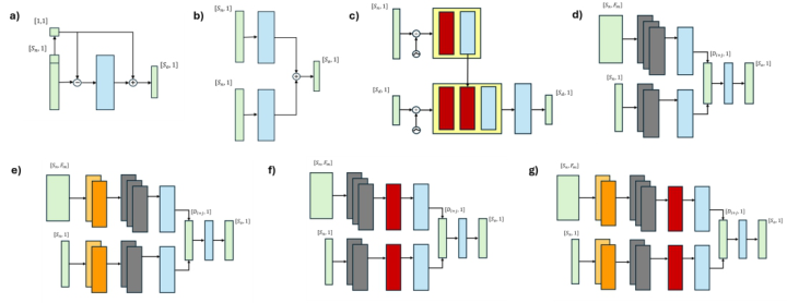
Opposite to the ARIMA model, the Transformer model has shown strong performance with long-term forecasting but has recently come under scrutiny for its handling of temporal information. It is also worth noting that the iterative predictions made by Transformer models lead to high computation costs, which are exacerbated for longer sequence predictions. This issue may compromise real-time application. Figure 1 shows a simplified version of the Transformer architecture applied in this study.
Based on the transformer model issues, Zeng et al. (2023) proposed two linear models to better handle temporal features. The first is a decomposition model, DLinear, that accounts for trends and seasonality in data. A second
variation is a normalization model, NLinear, that accounts for shifts in the distribution of data. The DLinear model decomposes initial input into a moving average component and a residual component before applying an individual linear layer to each, and then summing the outputs to obtain a final prediction. The NLinear model, on the other hand, normalizes the input by subtracting the last timepoint. It then processes the normalized input in a single linear layer before adding the last timepoint back into the output. Both architectures are also depicted in Figure 1.
Finally, the recurrent linear models that we tested are variations on a bi- directional GRU network (Cho et al., 2014). These models have a simpler architecture than LSTM models which makes them faster for inferencing. Recurrent networks are adept at handling temporal information due to their architecture but exhibit poorer performance when attempting to learn longer sequences. Consequently, we evaluated two variations on the GRU network. The first model variation included a self-attention module following the GRU layers and before the linear (prediction) layer. This self-attention procedure followed the same format as outlined in Wang et al. (2021). In this case, the last GRU layer’s cell output is treated as the query and the key, and values are treated as the full final layer output. Compared to the traditional approach, self-attention mechanisms can leverage the information across all cells at each sequence point and account for their relevance in the final prediction with negligible computational costs. The second variation involves incorporating a 1D convolutional neural layer (CNN; LeCun et al., 1998) prior to the GRU layers to extract local features in a dataset. In addition, a max pooling layer is incorporated to increase the robustness of the CNN by supressing sensitivity to noise in the input. However, this approach comes with a steep increase in computation costs during inference. The architectures for each of the model variations can also be seen in Figure 1. Sigmoid activation functions were applied at the final layer of each network to normalize outputs between 0 and 1. Additionally, each intermediate linear layer and convolutional layer included a normalization step and leaky rectified linear unit activation function (Maas et al., 2013) to improve robustness and introduce nonlinearity, respectively.
Initially, the perceptual load data from the multinomial classification model, consisting of three predicted class confidences, was found to be imbalanced. Specifically, instances of pilot underload represented only 10% of the total classifications. Meanwhile optimal and overload confidences encompassed 45% of the total classifications, each. Since pilot perceptual overload represents a potential safety critical event, the underload and optimal classification likelihoods were combined to counter the initially imbalanced dataset while preserving the critical overload perceptual load label. The fNIRS data, which was used in training the GRU models, was scaled for each processed sequence using a minmax scaler ranging from -1 to 1. The model input sequence consisted of the last 90s of data, while the forecast was the next 10s of perceptual load. The input was the confidence likelihood from the multinomial model for the pilot perceptual overload class (including fNIRS for GRU models). The complement of the overload confidence was used to predict the combined underload and optimal (i.e., not
Deep Learning Forecast of Perceptual Load Using fNIRS Data 17
overload) confidence. Past fNIRS data were not used with the linear, ARIMA, or Transformer models, as this would require additional modifications to the original models to properly account for these covariates, which falls outside of the scope of the present study.
During training, the 46 trials of data were split into six testing trials and 40 training trials. The training trials were further divided into five cross-validation folds (32/8 train/validation splits) to evaluate the generalization capabilities of each model. Regression loss metrics for the 5- fold cross validation step were analysed. In addition, the model classification performance was evaluated using the six test trials of data. A mean squared error (MSE) loss was used to train the models alongside an Adam optimizer (Kingma & Ba, 2014). The MSE loss measure was selected to heavily penalize predictions that result in large deviations from the original labels and improve model robustness for identifying large shifts in high load confidence. A combined loss function, considering both classification and regression loss, could be incorporated in model training to improve classification performance, however, the linear models were not capable of providing constrained outputs (i.e., through an activation function), which limited the adoption of classification loss functions in this study.
Figure 1: All model architectures. a) NLinear, b) DLinear, c) Transformer, d) base GRU, e) GRU with CNN, f) GRU with self-attention, g) GRU with CNN and self-attention. Tensor shapes are shown in green, linear layers are blue, encoder and decoder modules (for the Transformer) are yellow, GRU layers are grey (with each block denoting one layer), self-attention modules are red, and the CNN and max pooling layers are in light and dark orange, respectively.
RESULTS
Two analyses were conducted and reported here, including: (1) the average model regression loss across the validation datasets (Table 1); and (2) the model classification performance when applied to the test dataset (Table 2). The average computation time during inference, for each 10s forecast, is also reported in Table 1. The cross-validation performance is important to consider, as it represents model capability to generalize onto unseen data. It should be noted that the reported regression loss for the ARIMA model
(Table 1) simply reflects the regression loss across the same trials used for cross-validation for the deep learning models.
In terms of computational cost, the ARIMA and Transformer models produced the highest time costs. The ARIMA model has to be fit to the prior time data for any prediction. The iterative nature of the Transformer model requires that each future step is computed independently; hence, computation cost is dependent on the desired forecast length. In this study, we sought to predict 10s (100 timesteps) in the future. Consequently, the Transformer model was forced to create 100 predictions sequentially, as each prediction is iteratively leveraged to compute the next timestep. On the other hand, the simple architecture from the DLinear and NLinear models resulted in extremely quick computations. Finally, although the introduction of a CNN module did increase the computation cost for GRU models, the overall time cost is marginal.
From Table 1, it can be seen that the DLinear and NLinear models achieved the best regression performance across all folds while the Transformer model produced the worst generalization among all the deep learning models. Although the ARIMA model produced the worst overall loss for the validation set. However, this comparison is caveated by the fact that the ARIMA model does not use the same training methodology and is not aimed at minimizing an MSE loss function. Moreover, no GRU variation (i.e., +CNN, +SA, +CNN+SA) outperformed the basic GRU model by a considerable margin. In terms of classification performance across the test dataset, the GRU and NLinear models achieved the best results, both yielding a 0.80 weighted F1 score. The GRU model with self-attention underperformed when compared to the ARIMA model, resulting in a 0.73 macro F1 score and a 0.77 weighted F1 score.
Table 1. Average MSE loss for 5-fold cross validation, and average computation cost during inference.
Table available in the original PDF paper.
Metric ARIMA DLinear NLinear Transformer GRU GRU+SA GRU+CNN GRU+CNN+SA MSE Loss 0.0170 0.0139 0.0141 0.0158 0.0146 0.0146 0.0154 0.0145 Time (s) 0.225 4.25e−4 3.40e−4 0.905 0.0615 0.0590 0.0621 0.0605
Table 2. Classification performance for each model across the test dataset.
Deep Learning Forecast of Perceptual Load Using fNIRS Data 19
DISCUSSION AND FOLLOW-ON WORK The evaluation of model performance revealed several interesting findings. First, the best performing model in terms of regression loss during cross- validation was the DLinear model, which also produced one of the worst performances during classification. It was expected that the linear model capability to effectively predict future class confidences would extend to the capability to predict changes in classifications. Although regression performance could translate to classification performance, our results reveal that it is not a direct relationship. If the end-goal of modeling is to classify perceptual load, a different approach should be taken in terms of defining the model objective function. For example, a combined loss function, taking into account both classification and regression loss during training, could be applied to leverage continuous, granular observations on the target variable (i.e., perceptual load classification confidence) and penalize incorrect model predictions. This could be a weighted sum loss which takes cross-entropy and MSE loss into account during backpropagation.
A second finding to consider is the high computation cost of the Transformer model (and potentially other Transformer-based models) when performing real-time forecasting. The cost is primarily due to the fact that the perceptual load forecast follows the same timesteps as the original fNIRS measurement, which was recorded with 10Hz sampling. Hence, the model is required to perform ten predictions for each second that it attempts to forecast. A potential solution to this problem could involve changing the model output timesteps to a fraction of the original fNIRS response sampling rate. For example, the architecture could be structured to forecast every 10th timestep; thereby, forecasting the confidence value at each second. This would drastically reduce the iterative demand of the Transformer model during inference. It is also possible to down-sample the original data as model input. This would decrease the total number of parameters that each model has to learn and compute during inference. However, it is possible that when restricting these input dimensions (limiting available data for model training) the model performance would decrease. Consequently, achieving a balance of the number of input data features with model computation time is critical to real-time forecasting applications with Transformer models.
Referring to H1, although all deep-learning models outperformed the benchmark statistical (ARIMA) model, in terms of MSE loss, only certain models produced superior classification performance for the test dataset. Furthermore, the best deep learning models only marginally outperformed the benchmark. Although the deep-learning models proved effective for forecasting perceptual load, future research needs to further investigate the features of fNIRS and load classification data to leverage the capabilities of these models.
Counter to our original hypothesis, the GRU models did not achieve superior performance compared to the NLinear and DLinear models. This was surprising given the GRU model capability to account for the multinomial model overload classification confidence as well as the fNIRS data. It is possible that the relationship between the fNIRS features and
the load confidence is more complex than what a GRU model is able to capture. Hence, additional measures could be taken to better account for these covariates. One interesting approach, for example, would be to introduce a cross-attention mechanism, where information from the fNIRS data independently informs the attention scores, which are then applied to the load confidences.
Referring to H2, among the deep learning models, the Transformer model produced the worst performance. However, there have been several recent modifications to the Transformer model for applications to other time series domains, which could prove useful for forecasting pilot perceptual load, such as the Autoformer (Wu et al., 2021) and Informer (Li et al., 2021) models.
Lastly, it should be noted that no formal hyperparameter tuning was conducted in this study. Future studies should conduct a comprehensive examination of model tuning, for example, a grid search approach for each model across the cross-validation dataset. This would allow for more accurate comparisons of the optimal performance of each model. However, there is also a need to formulate an appropriate loss function that relates model training penalties to the end-goal of classification accuracy as a basis for hyperparameter tuning. The loss function should be used to guide the grid search for optimal model selection. In addition, model performance could be further boosted with computationally efficient pre-processing techniques, such as lifting schemes (Sweldends, 1996; Lee & Ko, 2011). These techniques can enhance the available information from raw input data.
CONCLUSION
Perceptual load forecasting has the potential to increase safe practices in piloting tasks by supporting monitoring systems that provide proactive cues to effectively direct pilot perceptions. This study explored a promising subset of forecasting models for specific flight tasks and highlighted potential limitations with current forecasting methodologies. Linear models proved to incur the least computational costs during inference and produced the lowest regression (MSE) losses during model cross-validation. On the other hand, GRU and NLinear models produced the best classification performance when evaluated on a test dataset consisting of several different trials of data. Although several deep learning models proved to be more effective than a statistical benchmark model, future improvements and variations to the models, processing techniques, and objective functions are yet to be explored. Finally, we also identified several future considerations for the development of effective perceptual load forecasting algorithms.
ACKNOWLEDGMENT
This work was partially funded by the U.S. Defense Advanced Research Projects Agency under contract #HR00112220004. Any opinions, findings, and conclusions or recommendations expressed in this paper are those of the authors and do not necessarily reflect these agencies’ views.
Deep Learning Forecast of Perceptual Load Using fNIRS Data 21
REFERENCES
Ayaz, H., Shewokis, P. A., Bunce, S., Izzetoglu, K., Willems, B. and Onaral, B., 2012.
Optical brain monitoring for operator training and mental workload assessment. Neuroimage, 59(1), pp. 36–47. Box, G. E., Jenkins, G. M., Reinsel, G. C. & Ljung, G. M., 2015. Time series analysis: forecasting and control. John Wiley & Sons. Cho, K., Van Merriënboer, B., Gulcehre, C., Bahdanau, D., Bougares, F., Schwenk, H.
and Bengio, Y., 2014. Learning phrase representations using RNN encoder- decoder for statistical machine translation. arXiv preprint arXiv:1406.1078. fNIR Devices LLC, n.d. fNIR Devices. Available at: https://fnirdevices.com/ [Accessed: 18 May 2024]. Grimaldi, N., Liu, Y., McKendrick, R., Ruiz, J. and Kaber, D., 2024, May. Deep Learning Forecast of Cognitive Workload Using fNIRS Data. In 2024 IEEE 4th International Conference on Human-Machine Systems (ICHMS) (pp. 1–6). IEEE. Harris, A. M., Eayrs, J. O. and Lavie, N., 2023. Establishing gaze markers of
perceptual load during multi-target visual search. Cognitive Research: Principles and Implications, 8(1), p. 56. Hochreiter, S. and Schmidhuber, J., 1997. Long short-term memory. Neural computation, 9(8), pp. 1735–1780. Kingma, D. P. & Ba, J., 2014. Adam: A method for stochastic optimization. arXiv
preprint arXiv:1412.6980. Lavie, N., 1995. Perceptual load as a necessary condition for selective attention.
Journal of Experimental Psychology: Human perception and performance, 21(3), p. 451. Lavie, N., Hirst, A., De Fockert, J. W. and Viding, E., 2004. Load theory of selective attention and cognitive control. Journal of experimental psychology: General, 133(3), p. 339. LeCun, Y., Bottou, L., Bengio, Y. & Haffner, P., 1998. Gradient-based learning applied to document recognition. Proceedings of the IEEE, 86(11), pp. 2278–2324. Lee, C. M. & Ko, C. N., 2011. Short-term load forecasting using lifting scheme and
ARIMA models. Expert Systems with Applications, 38(5), pp. 5902–5911. Maas, A. L., Hannun, A. Y. & Ng, A. Y., 2013. Rectifier nonlinearities improve neural network acoustic models. In Proc. ICML, 30(1), p. 3. Macdonald, J. S. and Lavie, N., 2011. Visual perceptual load induces inattentional
deafness. Attention, Perception, & Psychophysics, 73, pp. 1780–1789. McKendrick, R., Feest, B., Harwood, A. and Falcone, B., 2019. Theories and methods for labeling cognitive workload: Classification and transfer learning. Frontiers in human neuroscience, 13, p. 295. Nagle, F. and Lavie, N., 2020. Predicting human complexity perception of real-world
scenes. Royal Society open science, 7(5), p. 191487. Pang, X., Zhou, Y., Wang, P., Lin, W. and Chang, V., 2020. An innovative neural network approach for stock market prediction. The Journal of Supercomputing, 76, pp. 2098–2118. Peng, X., Jiang, H., Yang, J., Shi, R., Feng, J. and Liang, Y., 2022. Effects of Temporal
Characteristics on Pilots Perceiving Audiovisual Warning Signals Under Different Perceptual Loads. Frontiers in Psychology, 13, p. 808150. Raveh, D. and Lavie, N., 2015. Load-induced inattentional deafness. Attention, Perception, & Psychophysics, 77, pp. 483–492.
Sweldens, W., 1996. The lifting scheme: A custom-design construction of biorthogonal wavelets. Applied and Computational Harmonic Analysis, 3(2), pp. 186–200. Vaswani, A., Shazeer, N., Parmar, N., Uszkoreit, J., Jones, L., Gomez, A. N., Kaiser, Ł. and Polosukhin, I., 2017. Attention is all you need. Advances in neural information processing systems, 30. Wang, J., Grant, T., Velipasalar, S., Geng, B. and Hirshfield, L., 2021. Taking a deeper
look at the brain: predicting visual perceptual and working memory load from high-density fNIRS data. IEEE Journal of Biomedical and Health Informatics, 26(5), pp. 2308–2319. Wu, H., Xu, J., Wang, J. and Long, M., 2021. Autoformer: Decomposition transformers with auto-correlation for long-term series forecasting. Advances in neural information processing systems, 34, pp. 22419–22430. Zeng, A., Chen, M., Zhang, L. and Xu, Q., 2023, June. Are transformers effective
for time series forecasting?. In Proceedings of the AAAI conference on artificial intelligence (Vol. 37, No. 9, pp. 11121–11128). Zhou, H., Zhang, S., Peng, J., Zhang, S., Li, J., Xiong, H. and Zhang, W., 2021, May.
Informer: Beyond efficient transformer for long sequence time-series forecasting. In Proceedings of the AAAI conference on artificial intelligence (Vol. 35, No. 12, pp. 11106–11115). Zhu, R., Liao, W. and Wang, Y., 2020. Short-term prediction for wind power based on temporal convolutional network. Energy Reports, 6, pp. 424–429. Zhu, R., Wang, Z., Ma, X. and You, X., 2022. High expectancy influences the role of
cognitive load in inattentional deafness during landing decision-making. Applied Ergonomics, 99, p. 103629.
LISTED IN THE AHFE DIGITAL BOOKSTORE CATALOGUE
Explore the complete digital volume
Human Factors in Design, Engineering, and Computing
Read this individual research paper free through the original publisher, or explore the full digital proceedings book.
ISBN 978-1-964867-35-9
Explore this ISBN in the AHFE Bookstore ↗Listed in the July 2026 bookstore catalogue; search by ISBN to confirm current availability · Digital book purchase optional