Stefan Klug, Jonas Schmänk, Maximilian Moll, Stefan Pickl (2026). Strategic Defense against Hybrid Threats under Emerging Disruptive Technologies: A Stochastic Modeling Framework. In: Intelligent Human Systems Integration (IHSI 2026): Disruptive and Innovative Technologies. AHFE Open Access, vol. 200, pp. 207–216. https://doi.org/10.54941/ahfe1007080
The fundamental unpredictability of Emerging Disruptive Technologies creates profound strategic asymmetries in hybrid threats, as defenders must prepare for unknown capabilities while attackers exploit breakthroughs. This research introduces a new model to analyze how technological uncertainty transforms optimal strategies for defensive actors, proving essential for developing robust strategies as the pace of technological innovation accelerates and the window between innovation and weaponization narrows. In this work, technological uncertainty is modelled as a stochastic evolutionary process, focusing on the defender's challenge of resource allocation. Through a parametrized model design, the framework provides high customisability for different scenarios and technology-specific insights relevant for developing optimized allocations of defense resources. We compare a naive baseline resource allocation against an optimized allocation in a simulated scenario, showcasing the need for differentiated defense postures and showcasing the need for differentiated defense postures and illustrating a novel pathway for reasoning under deep technological uncertainty. The experiments show a significant superiority of technology-tailored resource allocations, reducing overall attack impact and planning uncertainty.
Hybrid threats now increasingly shape the security landscape. As Emerging and Disruptive Technologies (EDTs) – AI, biotechnology, quantum, autonomous systems – accelerate, the window between innovation and weaponization keeps shrinking. Capabilities can surface abruptly, propagate unevenly, and interact across domains, defeating deterministic forecast-first planning. Examples include novel AI-enabled cyber-attacks or disinformation campaigns (Giannopoulos et al., 2021). We analyze how this technological uncertainty changes defense decisions. Defenders must allocate scarce resources ex ante without knowing which technologies will become operational threats, while attackers can opportunistically exploit breakthroughs. Our aim is to provide a model to analyse acting under deep uncertainty. Therefore, we combine established modelling elements into a coherent stochastic model for analysing defence strategies under technological uncertainty.
Our approach models technology maturity as a stochastic process punctuated by rare breakthroughs, maps maturity to operational threat intensity via a simple and interpretable materialization function and quantifies how defensive investments attenuate those threats. A small of parameters governs (i) progress speed and volatility, (ii) activation thresholds and curvature in materialization, and (iii) defense effectiveness with diminishing returns, thus enabling scenario analysis, sensitivity checks, and portfolio- style allocation.
Our contributions are threefold: (1) a tractable jump-diffusion model of EDT maturation; (2) a transparent maturity-to-threat mapping with activation thresholds and (3) a defense effectiveness model linking budgets to residual exposures. Collectively, these support principled stress-testing across technological futures.
BACKGROUND
Work on technology diffusion traditionally models adoption as smooth S-curves, with the Bass model as the canonical baseline (Bass, 1969). However, survey evidence shows that real diffusion paths are heterogeneous – epidemic learning, legitimation, network effects, and cascades – so purely deterministic curves often miss regime shifts and discontinuities (Geroski, 2000).
To address these breaks, a second strand adopts stochastic models with jumps. Jump-diffusion frameworks capture both incremental drift and rare, high-impact shocks; Kou’s double-exponential jump-diffusion provides tractable heavy tails and asymmetry (Kou, 2002). Applied to adoption, these models argue that large, infrequent jumps are intrinsic to innovation – an especially apt description for EDTs (Teffahi, 2012). As maturing technologies create attack opportunities, security economics links evolution to defensive choices. On the spending side, Gordon-Loeb derive benchmark investment rules under diminishing returns (Gordon and Loeb, 2002). On the adversarial side, Stackelberg Security Games formalize budgeted defense against adaptive attackers, while formal security models and generic threat matrices supply structured state spaces and taxonomies-motivating separable baselines and many-to-many mappings from technologies to threats (Kar, 2018; Ryan, 2001; Duggan, 2007). Aggregating multi-dimensional residual exposures likewise benefits from convex, risk-sensitive measures that better reflect co-occurrence and tail losses than linear sums (McNeil, 2015). An allied dose-response debate offers intuition for mapping maturity to risk: linear no-threshold is conservative, whereas thresholded responses capture activation effects beyond a critical level (Wojcik and Zölzer, 2024).
Based on these strands, we couple a jump-diffusion process of EDT maturity with a parameterized materialization map and a budgeted defense allocation problem, enabling analysis across uncertainty regimes and retaining interpretability.
MODEL EDTs evolve stochastically and can generate novel threats at unpredictable times. Defenders allocate resources ex ante without knowing which EDTs will materialize into threats, while attackers may exploit EDTs opportunistically when advantageous.
State Variables and Spaces At time 0 t ≥ , the model is summarized by the triple ( ) , , t t w X T : the defender’s allocation w, the vector of technology maturities t X , and the induced threat intensities tT . Defense Portfolio Space. The defender allocates a fixed budget 0 B > across
n i n
Equations and mathematical formulas are available in the original paper PDF.
n defense categories, with a defense portfolio ( ) { } 1 : Technology State Space. The maturity of k EDTs at time t is given by k + = … ∈[Equation or mathematical symbol available in the original paper PDF].
( ) ( ) ( ) 1 k t t t X X , ,X Threat Space. Potential threats are represented by a vector k tT + ∈[Equation or mathematical symbol available in the original paper PDF], where each component captures the intensity of a particular attack vector.
Stochastic Technology Evolution Following Geroski (2000), we model latent technological maturity for each technology 1, , i k = … by a jump-diffusion process that accommodates both gradual progress and rare breakthroughs. Let ( )i t X ∈[Equation or mathematical symbol available in the original paper PDF] denote the (unbounded) latent maturity state. Each technology ( )i t X evolves according to a jump-diffusion process (Merton, 1976):
where ( ) , i t µ ⋅ is positive deterministic drift (baseline technological progress), ( ) , i t σ ⋅ the diffusion coefficient (continuous uncertainty), ( )i t W a standard Brownian motion, ( )i J the jump size sampled from a normal distribution, such when a breakthrough occurs and ( )i t N a Poisson process representing breakthrough events with intensity ( )i N λ , with the parameters of the probability distributions being technology-specific. ( ) 0 i X can be initialized with scenario- specific values to model various starting conditions.
This formulation captures both gradual technological progress and sudden, unpredictable breakthroughs.
Due to its positive deterministic component, ( )i t X tends to infinity. Under the observation, that eventually increasing technical maturity has diminishing impact on the actual applicability of a technology, a bounded function that is degressive after passing a certain threshold is included in the model as well. To address the applicability of the model in decision making process, we map the latent state to a bounded Technology Readiness Level (TRL) ( ) [ ] 0,9 i tY ∈ as an established concept in technology driven-contexts via a logistic function ( ) ( ) ( ) i t X i tY = Γ with technology-specific slope 0 ik σ > and midpoint
( ) :
[Equation or mathematical symbol available in the original paper PDF] , under the assumption, that for higher
1 9 1 exp
i t i k X x ⋅ i
[Equation or mathematical symbol available in the original paper PDF][Equation or mathematical symbol available in the original paper PDF] + −σ − [Equation or mathematical symbol available in the original paper PDF][Equation or mathematical symbol available in the original paper PDF] technical maturity ( )i t X , the effects on higher TRLs is diminishing.
Threat Materialization Function The realized threat vector at time t is given by ( ), t t T Y = Φ where : k k + + Φ → [Equation or mathematical symbol available in the original paper PDF][Equation or mathematical symbol available in the original paper PDF] maps the maturity levels of the k EDTs componentwise into k corresponding threat intensities. The function Φ may exhibit threshold or nonlinear effects, reflecting the fact that a technology only becomes threatening once its maturity level crosses a critical point.
A suitable threat materialization function for ( ) tY Φ is a nonlinear threshold function. This type of function effectively models the relationship between an EDT maturity and the intensity of its corresponding threat. The function captures the idea that a technology only becomes a significant threat once its maturity level exceeds a certain critical point.
Y Y Y
β α θ α β θ θ
, if 0, 0, 0, 0, if
Y
i i i i t t i t i i i i t i
[Equation or mathematical symbol available in the original paper PDF] ⋅ > [Equation or mathematical symbol available in the original paper PDF] Φ = > > ≥ [Equation or mathematical symbol available in the original paper PDF][Equation or mathematical symbol available in the original paper PDF] ≤ [Equation or mathematical symbol available in the original paper PDF] where iθ is the critical maturity threshold for the i-th EDT, i α is a scaling factor governing the post-threshold growth rate and iβ is an exponent that controls nonlinearity (if 1 iβ > , the threat intensifies at an accelerating rate). This piecewise function remains at zero until the maturity level ( )i tY surpasses the critical threshold iθ . Once past this point, the threat intensity materializes and increases according to a power law. This model is consistent with the observation that a technology (e.g., artificial intelligence) may pose negligible risks for some time, but once it reaches a certain level of sophistication, the associated threats (e.g., deepfakes, autonomous weapons) can grow rapidly.
Defense Effectiveness Model This section formalizes how defensive investments attenuate realized threats and how the remaining exposure is summarized into a decision-relevant loss. The model has two components: the Protection Function ( ) , t t P w T , which maps a defense portfolio and a threat profile into post-defense (residual) exposure per dimension and Residual Loss After Protection, which aggregates the residual vector [Equation or mathematical symbol available in the original paper PDF]( ) tT w into a scalar loss ( ) t L w via a chosen risk-sensitive aggregator. The next subsections detail these components.
Protection Function Given a defense portfolio k w D + ∈ ⊆[Equation or mathematical symbol available in the original paper PDF] and a realized threat vector k tT R+ ∈ , the protection function measuring the effectiveness of the budget vector in component i is defined by ( ) ( )
( ) ( ) ( ) ( ) t t t P w,T T 1 e
(time-invariant) allocation to defense dimension i, and 0 i C > is a sensitivity parameter (either a common scalar or technology-specific). Higher ( )i tP indicates better protection.
The full protection vector is ( )
( ) ( ) ( ) 1 , , , , , , k t t t t t t P w T P w T P w T = … which collects the effectiveness of each defense dimension against the realized threat profile tT . This specification serves as a tractable baseline that can be generalized to nonlinear mappings (see also Duggan, 2007).
Residual Loss After Protection Let k tT + ∈[Equation or mathematical symbol available in the original paper PDF] denote the realized threat vector at time t and ( ) , k t t P w T + ∈[Equation or mathematical symbol available in the original paper PDF] the
corresponding protection vector generated by defense portfolio w D ∈ .
The residual threat vector is then ( ) ( ) ( ) , , t t t t T w T P w T
( ) ( ) ( ) max{ , ,0} i i i t t t t T w T P w T = − [Equation or mathematical symbol available in the original paper PDF] for each component i. To evaluate overall damage, we introduce a loss aggregator : k r + + → [Equation or mathematical symbol available in the original paper PDF][Equation or mathematical symbol available in the original paper PDF] that maps the residual threat vector into a scalar loss (see also McNeil, 2015): ( ) ( ) ( ). t t L w r T w = [Equation or mathematical symbol available in the original paper PDF] The choice of aggregator r captures a decision-maker’s preferences: Linear form, ( ) r z z = α[Equation or mathematical symbol available in the original paper PDF] with some k + α ∈[Equation or mathematical symbol available in the original paper PDF], yields a weighted- sum baseline, while convex forms (e.g. norms or power functions) model risk aversion, cascading effects, or worst-case sensitivity across multiple threat dimensions.
Payoffs The defender chooses a static portfolio w D ∈ to minimize the expected discounted loss plus a (possibly convex) deployment cost:
( ) ( ) ( ) ( ) ñ
0 , D t
METHODS
We compare two static allocation rules, each choosing a single budget vector wat 0 t = , which is then held fixed over the horizon. Uniform allocation. A baseline that spreads the budget evenly across
Optimized allocation. In the given model, various techniques are applicable to derive optimized resource allocation. Since the detailed optimization of the model will be left for future work, the focus of this section is to showcase the general significance of optimization and to lay groundwork for future model iterations. The stochastic process is implemented in a discrete manner for simulation purposes (Glasserman, 2003), essentially making it a discrete Markov decision process. Subsequent studies will implement dynamic resource
allocation with sequential decision-making, thereby rendering reinforcement learning a feasible optimization approach. In order to derive an optimised static resource allocation in the current work, reinforcement learning is employed for the exploration of its general applicability. Therefore, a reinforcement learning agent with policy π is trained to maximise the expected discounted reward (negative loss). The observation is given by ( ) ( ) 0 0 , , t t Y Y θ Φ ; the action
is a continuous allocation projected onto D. At evaluation, the policy outputs , , t t w Y Y π θ = Φ , which is fixed for the a single one-shot allocation ( ) ( ) 0 0 rl
episode. In the current setup, a finite time horizon T = 10 is considered. We use Soft Actor-Critic (SAC) due its sample efficiency (Haarnoja, 2018).
All methods are evaluated by the same criterion, the expected discounted loss ( ) t
t t L w [Equation or mathematical symbol available in the original paper PDF][Equation or mathematical symbol available in the original paper PDF] δ [Equation or mathematical symbol available in the original paper PDF][Equation or mathematical symbol available in the original paper PDF] ∑ [Equation or mathematical symbol available in the original paper PDF] under the stochastic technology trajectories, with the cost ( ) c w of maintaining some budget allocation w being set to 0 and where the residual threat aggregator r is the unweighted sum of ( ) ( ) i tT w [Equation or mathematical symbol available in the original paper PDF] .
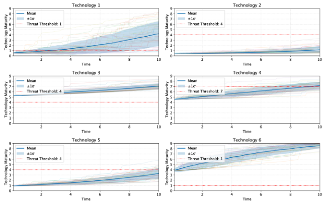
Figure 1: Trajectories of 200 sampled technology evolutions, given the initial set of parameters displayed in Table 1.
EXPERIMENTS AND RESULTS To assess the models capabilities and limitations, we have deployed the model for a varying set of randomly initialized parameters (see Appendix). The parameters set has been used in 200 simulation runs each to create technology and threat trajectories with 6 k = technologies, with initial technology maturity ( ) 0 i X initialized from a random uniform distribution. The uniform and RL-based budget allocation are evaluated against these simulated trajectories.
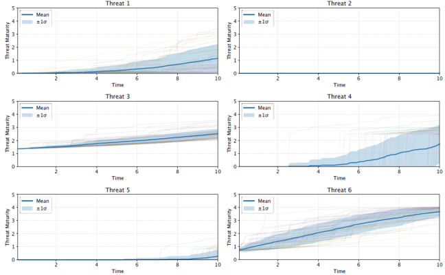
Figure 2: Trajectories of 200 sampled threat evolutions, based on the technology trajectories, given the initial set of parameters displayed in Table 1.
To assess the model capabilities, we used linear residual loss functions and a discount factor of 0.95 over a time horizon of 10 time steps. With the parameter set shown in Error! Reference source not found. the corresponding technology and threat trajectories displayed in Figure 1 and Figure 2 were simulated (see APPENDIX: OVERVIEW OF MODEL PARAMETERS for further parameters used in the simulation). A high flexibility to account for different evolution paths of EDTs can be observed, enabling the simulation of customized threat scenarios, thus addressing the need for customizable models that can serve as a foundation for decision-making under technological uncertainty.
Table 1: Model parameters used in simulation and respective budget allocations deviation.
Table available in the original PDF paper.
Threat i Parameter k σ 0.65 0.42 0.33 0.40 0.46 0.56
( )i J σ 0.48 0.49 0.46 0.17 0.12 0.33 Allocation uni w 1.67 1.67 1.67 1.67 1.67 1.67
RL w 1.87 0.09 2.63 2.65 0.08 2.67
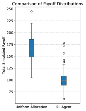
In the given parameter setup, the uniform allocation resulted in a higher expected total simulated payoff of approximately 156.94, with a standard deviation of 26.22. In contrast, the RL agent achieved a notably lower expected loss of approximately 100.58, with a standard deviation of 20.84 through its technology-specific budget allocation (see Figure 3).
Figure 3: Distribution of the total simulated payoff of 200 simulations for the uniform and RL-based allocation under the parameter set given in Table 1.
This suggests the RL agent’s learned strategy is more effective at minimizing loss in this dynamic threat environment compared to a naive uniform distribution. The lower standard deviation of the threat-specific allocation is especially insightful for risk-averse contexts. Notably, the coefficient of variation is 0.17 in the uniform allocation and 0.21 in the RL case. Specifically, technologies 3, 4, and 6 received the highest average allocations, while technologies 2 and 5 received the lowest. This non-uniform distribution aligns with the lower expected loss achieved by the agent, implying that tailoring the defense strategy based on the characteristics and evolution of individual technologies is crucial for minimizing overall risk.
In the current parameter setting, little budget is allocated to technology 4 despite its highly dynamic configuring parameters. As correctly predicted by the RL-agent, it does not reach the threat threshold in the investigated time interval, therefore not requiring any budget allocation at 0 t = . In a dynamic allocation setting, the defence vector would be expected to increasingly accommodate more budget for this technology for t Y with t 0 > . Overall, the base model demonstrates strong capability to describe a high variety of threat trajectories while also hinting at the need for optimized resource allocation strategies in environments under high uncertainty.
CONCLUSION
We have introduced a novel model paradigm to capture technological uncertainty in defensive postures under strategic asymmetry between defender and potential attackers, as it is typical in environments facing hybrid
Strategic Defense Against Hybrid Threats Under Emerging Disruptive Technologies 215 threats, thereby addressing growing needs of practitioners and researchers. The proposed model builds on clearly defined, but parametrized building blocks, namely a stochastic jump-diffusion-process to describe technological evolution including disruptive innovations leading to rapid advancements in a threat domain. To accommodate different thresholds of technologies to become relevant in an attack, a threat materialization is introduced and a defence effectiveness function that maps a defence budget allocation to specific threats. The final aggregated loss is analyzed based on chosen budget allocations. A budget allocated by a SAC-agent significantly outperformed a naïve baseline uniform allocation. The general applicability of the model to describe complex and stochastic technological evolution in various scenarios and the need for sophisticated defense strategies was therefore demonstrated.
The present framework takes a static, ex-ante view of defense allocation. A natural next step is to endogenize dynamic decision-making so that the defender updates allocations as evidence about technology maturation accumulates. Concretely, rather than choosing w once at 0 t = , future work will develop strategies that maps the available information tI (e.g., current TRLs tY estimated jump intensities, and recent threat realizations) to a budget-feasible allocation dynamically at each time t. Furthermore, in future work, empirically derived technology-specific parameters can be employed, to allow for near-real-world finding.
APPENDIX: OVERVIEW OF MODEL PARAMETERS Global and Simulation Controls
The stochastic process evolves with drift rates uniformly sampled from [0.01, 0.03], volatility from [0.01, 0.02], breakthrough intensities from [0.1, 0.8], and normally distributed jumps with means in [0.2, 0.8] and standard deviations in [0.1, 0.5].
Number of technologies 6 k = .
Defense Budget 10 B = .
Discount factor of loss function 0.95 δ = .
Threat and Defense Interaction
Threat materialization Φ: componentwise thresholded power law ( )
i tT with scales 0.05 i α = , exponents 2 iβ = , and thresholds iθ { } 0, ,8 ∈ … as in Table 1
Defense effectiveness ( ) ( ) , i t t P w T with parameter 0.5 C = SAC Hyperparameters (Stable-Baselines3):
Learning rate: 0.0008
Tau: 0.1
Batchsize: 512
Total time steps: 5000
Remaining parameters are default values
ACKNOWLEDGMENT
This work was partially realised with the collaboration of the European Commission Joint Research Centre under the Collaborative Doctoral Partnership Agreement No 36125.
REFERENCES
Bass, F. M. (1969). A new product growth model for consumer durables. Management Science, 15(5), 215–227. https://doi.org/10.1287/mnsc.15.5.215 Duggan, D. P., Thomas, S. R., Veitch, C. K. K., & Woodard, L. (2007). Categorizing
threat: Building and using a generic threat matrix (SAND2007-5791). Sandia National Laboratories. https://doi.org/10.2172/921121 Geroski, P. A. (2000). Models of technology diffusion. Research Policy, 29(4), 603–625. https://doi.org/10.1016/S0048-7333(99)00092-X Giannopoulos, G., Smith, H., Theocharidou, M., Cullen, P., Juola, C., Karagiannis, G.,
Kivisoo, K., Normark, M., Rácz, A., Schmid, J., & Schroefl, J. (2021). The landscape of Hybrid Threats: A Conceptual Model. Publications Office of the European Union. https://dx.doi.org/10.2760/44985 Glasserman, P. (2003). Monte Carlo Methods in Financial Engineering. Springer, New York. https://doi.org/10.1007/978-0-387-21617-1 Gordon, L. A., & Loeb, M. P. (2002). The economics of information security
investment. ACM Transactions on Information and System Security, 5(4), 438–457. https://doi.org/10.1145/581271.581274 Haarnoja, T., Zhou, A., Abbeel, P., & Levine, S. (2018). Soft actor-critic: Off-policy maximum entropy deep reinforcement learning with a stochastic actor. arXiv preprint arXiv:1801.01290. http://arxiv.org/abs/1801.01290 Kar, D., Nguyen, T. H., Fang, F., Brown, M., Sinha, A., Tambe, M., & Jiang, A. X.
(2018). Trends and applications in Stackelberg security games. In T. Başar & G. Zaccour (Eds.), Handbook of dynamic game theory (pp. 1–47). Cham: Springer. https://doi.org/10.1007/978-3-319-27335-8_27-1 Kou, S. G. (2002). A jump-diffusion model for option pricing. Management Science, 48(8), 1086–1101. https://doi.org/10.1287/mnsc.48.8.1086.166 McNeil, A. J., Frey, R., & Embrechts, P. (2015). Quantitative risk management:
Concepts, techniques and tools (Rev. ed.). Princeton, NJ: Princeton University Press. Merton, R. C. (1976). Option pricing when underlying stock returns are discontinuous.
Journal of Financial Economics, 4(1), 125–144. Ryan, P. Y. A. (2001). Mathematical models of computer security. In R. Focardi & R. Gorrieri (Eds.), Foundations of security analysis and design: Tutorial lectures (pp. 1–62). Berlin, Heidelberg: Springer. https://doi.org/10.1007/3-540-45608-2_1 Teffahi, B. (2012). On the technology adoption with the double exponential jump
diffusion process. Working paper, Real Options Conference. https://realoptions. org/openconf2012/data/papers/52.pdf Wojcik, A., & Zölzer, F. (2024). The scientific nature of the linear no-threshold (LNT) model used in the system of radiological protection. Radiation and Environmental Biophysics, 63. https://doi.org/10.1007/s00411-024-01092-1
LISTED IN THE AHFE DIGITAL BOOKSTORE CATALOGUE
Explore the complete digital volume
Intelligent Human Systems Integration (IHSI 2026): Disruptive and Innovative Technologies
Read this individual research paper free through the original publisher, or explore the full digital proceedings book.
ISBN 978-1-964867-76-2
Explore this ISBN in the AHFE Bookstore ↗Listed in the July 2026 bookstore catalogue; search by ISBN to confirm current availability · Digital book purchase optional