Viktor Dolia, Igor Ivanov, Iaroslav Sanko, Denis Pankratov, Yevhen Kush (2022). Forecasting of Evolution System the Driver – A Vehicle – Transport Network – Environment. In: Advances in Human Aspects of Transportation: Part III. AHFE Open Access, vol. 17. https://doi.org/10.54941/ahfe100759
The purpose of the article is method perfecting of the evolutionary probabilistic modeling that takes into account changes in the environment and the impact on all members of «the driver – a vehicle – transport network – environment». This allows to predict the evolution of any technical system with a variable environment. In work was established that the periods duration at locked state within each evolution stage of the system decreases. The disconnected state periods duration increases according to geometric progression. Also, the environment impact does not release system was determined. The environmental factors was analyzed. The gross domestic product was set like the key factor. As a result, any changes the transition environment probability in a given factual situation. It is possible to get a new model for determining the predictive values. Completed in 2006 forecast the evolution of «the driver – a vehicle – transport network – environment» (for example, in Kharkiv tram) had a valid value. As confirmed prediction verification data of 2007-2012 years. Transition probability model from the initial state to the final is refined. The proposed method allowed to apply evolutionary probabilistic modeling including a changing environment. This allows obtaining more reliable predictions of the evolution of any technical system.
As a consequence of the scientific and technological progress, the modern evolutionary processes under way in the society undergo sweeping changes. They are conditioned by a large scale of production, a variety of production spheres, expansion of inter-branch ties, shortening of the period of the scientific and technical achievements implementation etc. This, in its turn, encourages scientists in various fields to join their forces in order to solve the common issues of development of large-scale systems and their subsystems (Grinin and Korotayev, 2013).
The major problem emerging in the course of discussion of urgent issues and making decisions regarding them is analyzing certain stages of the system development, which gives rise to new standpoints and ways to consider the problems emerging during the systems’ functioning. The adequate results can be obtained only with the use of the modern system analysis methods, based on consideration of the entire evolutionary way of the system existence (Grigorov et al., 2006).
FORMATION OF THE FUNDAMENTAL PRINCIPLES OF THE EVOLUTIONARY- PROBABILISTIC MODELING Formation of the system evolution
The study revealed that any system (biological, technical, social, economic etc.) passed through the following stages in the course of development (Fig. 1): formation; growth; permanent functioning; recession (Rozovskiĭ 1990).
stable functioning
growth
recession
formation
System evolution time
Figure 1. System evolution milestones
Figure available in the original PDF paper.
The subject of the studies conducted by many scientists was not only the milestones proper, but the points of transition from one state to another. Thus, the fundamental principles of the “self-organization” system were formed, determining that any diversity of choices needs a transfer or processing of the amount of information, equal to this choice. That is, the choice is made in accordance with certain regularities that need to be studied (Park 1962).
This theory is reflected in the paper, which defines that the system is functioning under the influence of the internal and external stimuli. The former emerge during the collision between the elements, the latter – under the influence of external forces. That is, the processes of the state transition are permanently under way in the systems (Thompson 2011).
Using these approaches, Ie.V. Gavrilov in his paper (Grigorov et al., 2006) formulated the principles of evolution of the system “a man – an automobile – a road – natural space”. The heart of the theory is that two needs are satisfied in the course of any activity: the need in determinacy and the need in activity of the interaction with the environment.
It was found that, when the need in activity of the interaction with the environment is satisfied, the system is organizationally open. And, vice versa, when the need in determinacy is satisfied, the system is closed and realizes potential capabilities of the means of activity. Therefore, the cyclic cause-effect trajectories are changed in the course of the system evolution (Lynnyk 2013).
The technique of the long-range forecasting in accordance with the evolutionary-probabilistic method includes the following stages (Grigorov et al., 2006): 1) analysis of the system (parameter) historical development; 2) building an experimental regressive dependence; 3) experiment reproducibility verification; 4) evaluation of the intervals of the closed and open states of the objects under investigation (state lags); 5) selection of the models of the process’ deterministic components for the closed and open object states; 6) calculation of the model coefficients; 7) model adequacy evaluation; 8) using the obtained model for forecasting; 9) forecast accuracy assessment; Human Aspects of Transportation III (2022)
10) forecast verification (checking the forecast validity on similar objects using other methods).
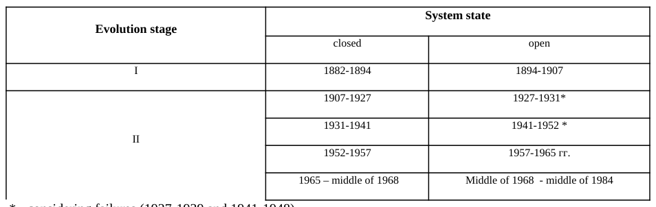
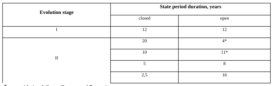
Determination of evolution of the tram traffic volume in the city of Kharkiv According to the long-term forecasting using the evolutionary-probabilistic method, the stages of the evolution of the system and the periods of the closed and open states and their duration were determined (Table 1-2).
The duration of the closed state periods within each state of the system evolution decreases, and the duration of the open state periods increases in the geometric progression.
Equations and mathematical formulas are available in the original paper PDF.
2 , (1)
р⋅2, (2)
tn+1
з,tn+1
where tn
з – duration of the period of stable growth of the traffic volume (closed state), years; р – duration of the period of the traffic volume stabilization (open state), years.
tn
р,tn+1 It is seen from Table 2, that at tn
з→0 and tn
Table 1: Sequence of the closed and open state periods in evolution of the tram traffic in the city of Kharkiv
* - considering failures (1927-1929 and 1941-1948)
Table 2: Duration of the closed and open state periods in evolution of the tram traffic in the city of
Kharkiv State period duration, years
* - considering failures (2 years and 7 years)
Based on results of assessment of maximum entropy of the system parameters, the time series (development series) is built Hmax=f (t) . Using the data of the tram traffic volumes, the time series of the tram development in the city of Kharkiv was determined and built (Fig. 2) (Yevtushenko 1983, Chmyhalо 2007).
5 6 7
2 3 4
Maximum entropy, units
Максимальна ентропія, од.
1880 1900 1920 1940 1960 1980 2000 2020 Роки
Years
Figure 2. Time series of the change of the tram traffic volume in the city of Kharkiv Analysis of the time series of the maximum entropy (Fig. 2) allowed detecting another abnormal situation, namely, reduction in the traffic volume in 1990, not accompanied by transition from the closed to the open state. If we follow the logic of the method of the evolutionary-probabilistic modeling, in 1990, a trend of the traffic volume growth or a transition to the open state shall persist till 1994.
Figure available in the original PDF paper.
Based on the information about the volume of the tram passenger traffic in 1984 to 1994, the system is found to be in the closed state, and a “jump” under the influence of the environment is observed.
It follows from the mathematical model of forecasting of the characteristics of the system “a man – an automobile –a road – a near-ground space” in the closed state, that the quantitative characteristic of the system component are determined using the probabilistic indices (Grigorov et al., 2006) X(t)=Xoq(t )+X з p(t) , (3) where X(t) – the current quantitative characteristic of the system component; Xo – the quantitative characteristic of the component with t=0; X з – the specified characteristic of the component (rate of state); q(t ) – the probability of the system component non-transition to the given state;
p(t) –the probability of the component transition to the given state.
The probabilities of transition of the components of the system “a man – an automobile –a road – a near-ground space” to the given state in relationship (3) are expressed from the equation of the system components’ dynamic equilibrium
dΔP
dΔP
ч
сер.ч
сер.ч
ч
сер.ч
a
сер.a
сер.a
a
сер.a
ΔP
ΔP
ΔP
ΔP
ΔP
ΔP
ΔP
ч
a
ч
c
a
ч
д
a
c
{
a
д
ч
c
ч
д
a
c
4) where ΔРч, ΔРа, ΔРд – variation of the probabilities of a man, an automobile and a traffic environment transition from the actual state to the given state; ΔРс – variation of the probability of the environment transition from the actual state to the given state; Qч,Qa,Qд – absolute organizations of the man, the automobile and the environment; Qсер.ч,Qсер.а,Qсер.д – rates of the absolute organization of the man, the automobile and the environment, respectively; Сч,Са,Сд – organizational capacity of the man, the automobile and the environment, respectively.
Solution of the differential equation system (4), with no changes in the system environment (weather-climatic, social and economic conditions), i.e. ΔРс =0, takes the form:
С
λ
λ
λ
λ
0M 0
1 τ
1 τ
з
1 τ
1 τ
з
Р
(e
−e
(e
−e
{
λ
λ
(5) where Рч, Ра, Рд− probabilities of the man, the automobile and the environment transition from the actual state to the given state, respectively; С0 ,С1,С2 – arbitrary constants depending on initial conditions; λ1 – characteristic equation root; τ – non-dimensional time; τ з – non-dimensional state lag.
Therefore, it is necessary to determine the environmental factors and their influence on changes in the volumes of the tram passenger traffic in the periods of the stable growth, i.e., when the system is in the closed state.
FORECASTING THE EVOLUTION OF THE URBAN PASSENGER SYSTEM Determination functions of the environmental changes
It was determined that the quantitative characteristic of the system component in future shall be found by relationship (3), and the respective probability of the system components transition to the given state – by relationships (4)-(5). If expression (4) is simplified, we will have the situation, when ΔРе=ΔРс , (6)
where ΔРе – variation of the probability of the system component transition from the initial to the finite state; ΔРс – variation of the probability of the environment transition from the initial to the final state; Based on the terms of the adequacy between the system elements and the environment, expression (6) will take the form:
kн ΔРе=ΔРс . (7) Therefore, expression (7) makes it possible to determine the degree of the interaction between the system element and the environment. For this purpose, the actual values of the environmental factors in the period under study shall be determined, and after that the distribution factor and the distribution function and the probability variation shall be found.
The gross domestic product is a more global and integral indicator reflecting effectiveness of the economy and social medium functioning (Hens and Schenk-Hoppe 2009, Galeeva 2007, Sun and Lynch 2008).
To reflect the gross domestic product distribution in the society, let us calculate the GDP per capita in US dollars and represent it graphically (Fig. 3).
Figure 3. GDP per capita distribution in US dollars
Figure available in the original PDF paper.
In this case, the probability of the environment transition from the actual status to the given one will take the following form:
−t . (8) Then, the variation of the probability of the environment transition from the actual state to the given one will take the form:
−t−1 . (9) The conducted study of determination of the variation of the municipal electrical tram environment in Kharkiv revealed that the main index was the GDP per capita in US dollars. For further calculations, relationship (9) shall be substituted in differential equation system (4), and the probability of the system element transition from the initial to the finite state shall be determined.
Determination of the urban passenger system evolution (by the example of tram) To solve this problem, it was proposed to substitute the studied variation of the probability of the environment transition from the initial to the finite state (9) in the right part of the differential equation system (4). Therefore, the differential equation system for the transport system of the urban passenger traffic will take the form:
dΔP
dΔP
п
сер.п
сер.п
п
сер.п
тз
сер.тз
сер.тз
тз
сер.тз
ΔP
ΔP
(te
ΔP
ΔP
ΔP
(te
п
тз+
тз
п+
м)−
{
тз
м
п
c
п
м
тз
c (10) where ΔРп, ΔРтз, ΔРм , ΔРс – variation of the probabilities of a passenger, a vehicle, a network and environment transition from the initial state to the finite state;
Qп,Qтз,Qм – absolute organizations of the passenger, the vehicle and the network, respectively; Qсер.п,Qсер.тз,Qсер.м – rates of the absolute organization for the passenger, the vehicle and the network, respectively; Сп,Стз,См – organizational capacity for the passenger, the vehicle and the network, respectively.
The partial solution of the system (10) will take the form:
−0,62τ
−1,38τ
−τ
−τ
−τ
−0,61τ
−1,38τ
−τ
−τ
−0,62τ
−1,38τ
−τ
{Р
−0,71e
−0,54τ+4,7e
⋅τ
+0,79τe
{P
+1,04e
+5,1e
{P
−0,74e
−0,68τ−0,01e
⋅τ
п
тз
м
(11) Upon finding the probabilities of the system elements’ transition from the initial to the finite state in such manner, they shall be verified when determining the theoretical values of the tram traffic volumes.
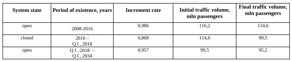
Using the empiric formulas to estimate the increment rates for the traffic volumes and duration of the closed and open state periods, the initial and finite values of the characteristic values in different periods of the system existence was forecasted (Table 3). The forecast of the volume of tram passenger traffic in the city of Kharkiv till 2034 is shown in Fig. 4.
Table 3: The forecast of the initial and the final values of the traffic volumes in different periods of the system existence Final traffic volume, System state Period of existence, years Increment rate Initial traffic volume, mln passengers mln passengers open 2008-2016 0,986 116,2 114,6
300
250
200
150
Passenger traffic, mln pass
100
50
1880 1900 1920 1940 1960 1980 2000 2020 2040 0
Year
Figure 4. Forecast of the volume of the tram passenger traffic in Kharkiv till 2034:
Figure available in the original PDF paper.
- theoretical values of the traffic volume; - actual values of the traffic volume.
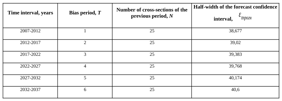
The confidence corridor of dispersion of the weighted average of the passenger traffic volume for the forecast period corresponding to the confidence probability Рд=0,95 , is given in Table 4.
Table 4: Confidence corridor of the forecast of the passenger tram traffic volume in the city of Kharkiv Half-width of the forecast confidence Time interval, years Bias period, Т Number of cross-sections of the previous period, N interval, εtпрогн
The upper limit of the confidence corridor can be treated as the optimistic forecast of the passenger traffic volume, the lower one – as the pessimistic forecast.
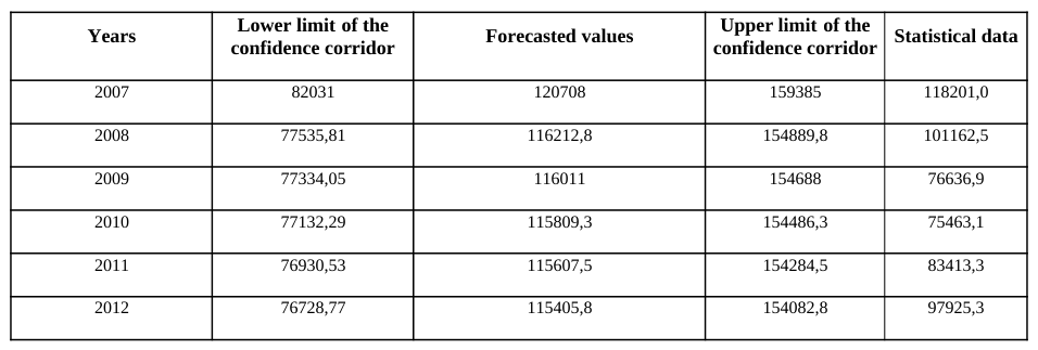
To verify the elaborated forecast, the forecast data (Fig. 4 and Table 4) and statistical data were taken and the assessment was made (Table 5).
Table 5: Verification of the forecast of the traffic volume for the period of 2007-2012 Years Lower limit of the confidence corridor Forecasted values Upper limit of the confidence corridor Statistical data
CONCLUSIONS
The forecast of the evolution of the urban passenger transport system, elaborated in 2006 (by the example of tram in the city of Kharkiv) was proven by verification based on the data of 2007-2012 (Table 5). All actual values are within the lower limit of the confidence corridor and the forecast data. It is explained by the economic situation in the region and the country as a whole in 2007-2012. Therefore, the method of the evolutionary-probabilistic modeling, in particular, the refined model (8)-(10), can be applied to describe evolution of the system «the driver – a vehicle – transport network – environment» with a variable environment.
REFERENCES
Chmyhalо, M. (2007), Statistical Yearbook: Kharkov region in 2006. Department of Statistics in the Kharkiv region. Chmyhalо (Ed.). 560 p. Departure (transport) of passengers by public transport Website:
http://kh.ukrstat.gov.ua/index.php/vidpravlennia-perevezennia-pasazhyriv-za-vydamy-transportu- zahalnoho-korystuvannia Galeeva, E. (2007), “Synergetic model GDP forecasts RUSSIA”, in: Problems of Modern Economics, Scientific and Production Company "ROST". No. 4. pp. 52-57 GDP per capita Website:
https://www.google.com.ua/publicdata/explore? ds=d5bncppjof8f9_&met_y=ny_gdp_mktp_cd&idim=country:UKR&dl=uk&hl=uk&q= %D1%81%D1%82%D0%B0%D1%82%D0%B8%D1%81%D1%82%D0%B8%D0%BA %D0%B0%20%D0%B2%D0%B2%D0%BF#! ctype=l&strail=false&bcs=d&nselm=h&met_y=ny_gdp_pcap_kd&scale_y=lin&ind_y=false&rdim=region&idim=country: UKR&ifdim=region&hl=uk&dl=uk&ind=false Grigorov, M. Gavrilov, E. Grigorov, T. Dolya, V. (2006), Prediction of the design characteristics of the design and operation of highways. Naddnepryanochka. 192 р. Grinin, L. Korotayev, A. (2013), Evolution: Development within Big History, Evolutionary and World-System Paradigms.
Uchitel Publishing House. 304 р. Hens, T. Schenk-Hoppe, K. (2009), Handbook of Financial Markets: Dynamics and Evolution: Dynamics and Evolution.
Elsevier. 608 р. Lynnyk, І. (2013), “Experimental evaluation of state dynamics of system«driver – vehicle»”, in: Аudit process of production and reserves, Тechnological center. Volume 6 No. 6(14). pp. 6-8 Park, R. (1962), Principles of Self-organization: Transactions of the University of Illinois. Symposium on Self-organization. New
York, Paris. 541 р. Rozovskiĭ, B. (1990), Stochastic Evolution Systems: Linear Theory and Applications to Non-Linear Filtering. Kluwer. 315 р. Sun, J. Lynch, T. (2008), Government Budget Forecasting: Theory and Practice. CRC Press. 664 р. Thompson, J. (2011), Organizations in Action: Social Science Bases of Administrative Theory. Transaction Publishers. 192 р. Yevtushenko, S. (1983), Relay in safe hands. Prapor. 112 р.
LISTED IN THE AHFE DIGITAL BOOKSTORE CATALOGUE
Explore the complete digital volume
Advances in Human Aspects of Transportation: Part III
Read this individual research paper free through the original publisher, or explore the full digital proceedings book.
ISBN 978-1-4951-2099-2
Explore this ISBN in the AHFE Bookstore ↗Listed in the July 2026 bookstore catalogue; search by ISBN to confirm current availability · Digital book purchase optional