Andrew McGordon, Stewart Birrell, John Poxon, Paul Jennings (2022). Comparison of Fuel Economy over Different Drive Cycles Each Having the Same Average Speed. In: Advances in Human Aspects of Transportation: Part III. AHFE Open Access, vol. 17. https://doi.org/10.54941/ahfe100743
The fuel economy of a vehicle is known to be highly dependent on its average speed during driving, with a maximum in fuel economy being present at around 40-50mph. Comparatively little work has been done on the investigation of how fuel economy varies for the same average speed. In this paper we report a theoretical simulation study of nine drive cycles each having the same average speed. The fuel economy for a typical C-segment vehicle varied from 37.3 to 74.4mpg for the nine drive cycles studied. Of the various metrics considered, standard deviation of speed, appears to be the most promising to explain the range of fuel economy. The results have important implications for transport planners, local authorities and national governments who rely on emissions predictions derived from vehicle average speeds. This research highlights the issues associated with this approach.
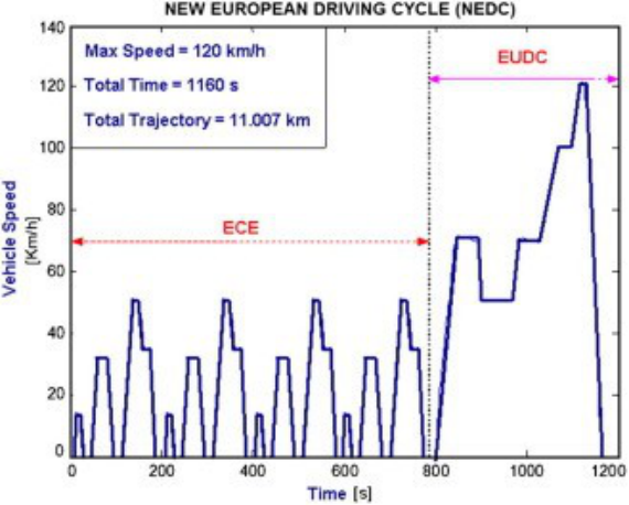
It is widely reported that new vehicle emissions are decreasing for both local air quality related emissions (for example Nitrous Oxides (NOx), Particulate Matter (PM), Hydrocarbons (HC) and Carbon Monoxide (CO)) and CO2 emissions. In the UK new car emissions have fallen by 26% from 2000 to 2012 (SMMT, 2013). In the European Union, the standard test cycle for legally binding local emissions measurements is the New European Driving Cycle (NEDC), and in the US it is the EPA Federal Test Procedure (FTP) tests. In recent years the NEDC has been used to derive a vehicle’s fuel economy and CO2 emissions as well as its local emissions performance. For a given fuel type (gasoline or diesel), CO2 emissions and fuel economy can be considered to be directly related, (DEFRA, 2013). The NEDC test consists of 4 repeated low speed cycles forming the urban phase of the drive cycle, and a higher speed extra-urban part of the drive cycle. There are no vehicle auxiliaries used such as lights, wipers or entertainment systems, and the NEDC has zero gradient. Figure 1 shows the NEDC drive cycle of speed versus time and provides detail of the drive cycle length and maximum speed; the average speed over the NEDC is 21mph.
Figure 1. Speed-Time profile for the EU Certification Drive Cycle (NEDC)
Results reported from this drive cycle are used by manufacturers, businesses and consumers to compare between vehicle types over this defined usage. The drive cycle has come in for criticism since it is clearly an idealised drive cycle, and it is not considered to be sufficiently representative for modern vehicle drive cycles (Andre, 2004). Various driver behaviour studies have shown that the acceleration rates of the NEDC are considerably lower than the acceleration rates seen in real world driving. This can be one of the contributory reasons why real world fuel economy is generally seen to be lower than the certification test values for individual vehicles (Mock et al, 2012).
Whilst the NEDC drive cycle is used by vehicle manufacturers to determine single vehicle emissions, a different approach is required for governments and local authorities. For example, governments are interested in greenhouse gas emissions to track progress against country level targets. It is interesting to note that although new car CO2 values have fallen by 26%, CO2 emissions from cars have fallen by only 16% over the same period (UK Government Statistics, 2013). This could be due to the issues with driver behaviour noted above, but also that these figures consider the whole car parc rather than just new vehicles. Local authorities are interested in the emissions in their area (NAEI, 2013) and for traffic planning purposes of an aggregated group of vehicles travelling over a particular stretch of road. This could amount to tens of thousands of vehicles per hour for arterial routes. Local authorities are particularly interested in local emissions such as CO, HC, NOx and PM, but also need to estimate CO2 emissions from transport. Currently, in the UK, emissions factors are defined in terms of average vehicle speed for a trip (Barlow et al., 2009). An example equation is reproduced below :
Equations and mathematical formulas are available in the original paper PDF.
where E is the emission rate in g/km v is the average speed of the vehicle in km/h
a to j and x are average speed based coefficients Numerous macroscopic traffic modelling approaches exist with the aim to determine vehicle speeds at a macro level. Approaches such as SATURN (van Vliet, 1982) and PARAMICS (Laird et al. 1999) assign high level parameters to individual vehicles, such as driver aggressiveness, following distance and overtaking behaviour. Many instances of these individual vehicles are then used to mimic traffic flows over particular sections of road. Macroscopic vehicle- to-vehicle interactions are captured and consequently vehicle speed profiles can be generated. These speed profiles are averaged and are used to lookup the expected steady state fuel consumption of reference vehicles in the models, and thus generate a macroscopic value for the fuel consumption, and hence the related CO 2 emissions. This approach is excellent for determining vehicle flows and congestion, but can only offer an approximation of vehicular emissions from traffic as the data is so aggregated. Due to the large number of vehicles involved, traffic planners use models which tend to average out the effects of individual vehicles and drive cycles. The emissions calculated from these models utilise specific emissions factors which are based on average vehicle speeds along specific “links” of road.
Barlow and Boulter (2009) conclude that the average speed approach to determining vehicle emissions provides results that are “reasonably accurate characterization of total emissions of road transport”. However the report also notes that emissions defined as functions of average speed may not be the best approach in some circumstances. This becomes particularly apparent for specific, small scale, traffic interventions such as the effect of changing traffic light phasing.
There has been much work characterising the effect that average speed has on fuel economy with the accepted maximum in fuel economy occurring at 40-50mph as this optimises the trade-off between overcoming rolling road resistance and increasing wind resistance, see for example Andre and Hammarstrom, 2000, and El-Shawarby et al., 2005. However, it is not only the average speed of the journey that has an effect on fuel economy, but also the specific nature of a drive cycle (Joumard et al, 2000). Of particular interest are the speed and acceleration profiles, which can vary widely in the real world and yet still give a relatively narrow spread in average speed attained. Clearly there are a large number of ways a vehicle can generate a particular average speed. The aim of this manuscript is to quantify the magnitude of the variation in fuel economy of a given vehicle over a range of drive cycles each having the same average speed but different speed-time profiles. This will help local and national governments more accurately predict and record both CO2 and local emissions. This manuscript presents a structured approach to investigate this.
The effect of nine different drive cycles on fuel economy was investigated, each with an identical average speed of 25 mph and identical start and end speeds. The 25mph average speed is representative of driving during morning rush hour on A-roads in the England (Department for Transport Statistics, 2013); this allows vehicle speeds from zero up to a maximum of 60mph.
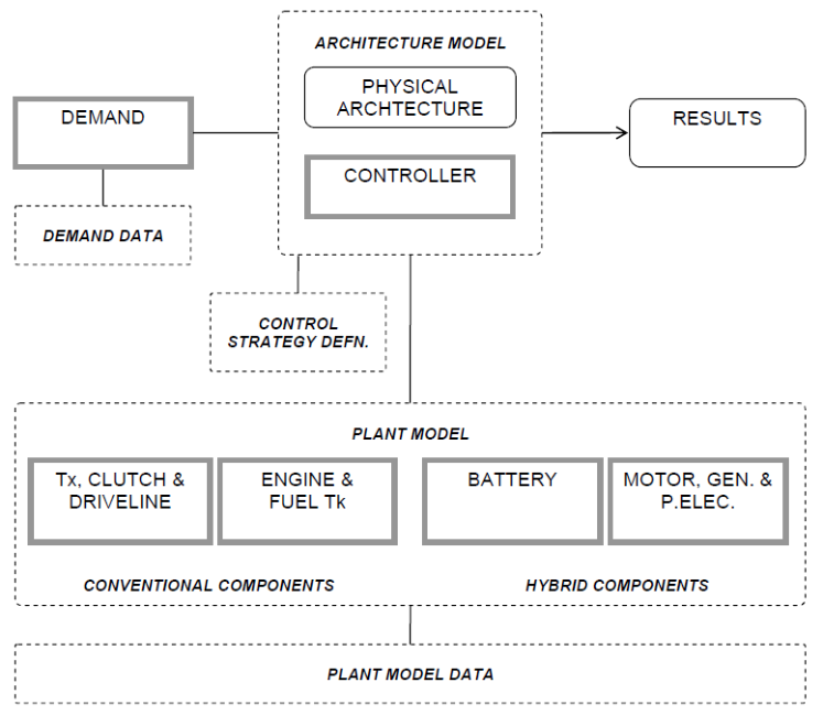
SIMULATION METHOD In order to determine the effect that a drive cycle has on fuel economy a standard vehicle and simulation package must be chosen. In this case a C-segment (for example, Ford Focus or Volkswagen Golf) 1.6ℓ Euro IV conventional petrol engined vehicle with 5 forward manual gears was chosen. The vehicle modelling package chosen to perform the simulations was WARPSTAR (Walker et al, 2006.), a hybrid architecture modelling package, which can also be used for conventional, hybrid and electric vehicles. Figure 1 shows a schematic of the WAPRSTAR structure for this study which has been used previously to study vehicle fuel economy (see for example, Cheng 2010). The inputs to the simulation are vehicle data and a speed-time drive cycle and the output in this case is fuel economy and CO2 emissions.
Figure 2. Schematic of the Generic Modelling Structure, WARPSTAR
Nine drive cycles were used in this work and are a combination of real world and artificially generated drive cycles. Importantly, all of the drive cycles are of exactly the same length, 2 miles, and have exactly the same average speed of 25mph; no gradients are included in the drive cycles. The vehicle speeds range from zero to 53mph, and the drive cycles range from constant speed to highly dynamic drive cycles. Figure 3 shows the drive cycles used in this study, with speed (red) and distance (green) plotted against time.
Figure 3. Detail of the Nine Drive Cycles Investigated
Figure available in the original PDF paper.
The vehicle was exercised over these drive cycles with gear change points being determined based on vehicle speed and vehicle torque demand. The gear change strategy was consistent across all drive cycles. Hot engine fuel consumption data was used throughout so that effects of engine warm up rate with load could be eliminated.
RESULTS AND DISCUSSION
For the nine drive cycles the predicted fuel economy outputted form the WARPSTAR simulation ranged from 37.3 to 74.4 mpg (imperial), a factor of approximately two difference (Table 1). The most visually dynamic drive cycles (Real-world 1 and Saw-tooth) have the lowest fuel economy indicating that drive cycle dynamics have an important influence on fuel economy. Although there was expected to be some variation of fuel economy with drive cycle dynamics for the same average speed, the magnitude of this variation is somewhat surprising. Also shown in Table 1 is the variation of fuel economy with standard deviation of speed of the drive cycle. The data indicates a general dependence of fuel economy increasing with decreasing standard deviation of speed, i.e. the reducing dynamic nature of the drive cycle. The reduction of the description of a drive cycle to one descriptor, standard deviation of speed, is an over simplification but there does appear to be an interesting relationship. Johansson et al. (1999) showed certain characteristics of driving behaviour that were significantly correlated with good fuel economy, including avoiding unnecessary stops. In the context of this paper reducing stops and keeping a consistent speed profile will relate to a reduction in SD of speed.
Table 1. Fuel economy of different drive cycles, and sample drive cycle description parameters
When shown graphically as in Figure 4, it is possible to consider the relationship between standard deviation of speed and fuel economy as potentially consisting of two regimes. The first regime can be considered to consist of an area of approximately constant standard deviation of speed (from 14.51 to 17.74 mph) and considerably varying fuel economy (from 37.3 to 65.8 mpg). The second regime consists of an area of approximately constant fuel economy (from 65.3 to 74.4 mpg) for considerably varying standard deviation of speed (from 0 to 14.51 mph). This could indicate that below a certain vehicle demand, fuel economy varies only slightly with the standard deviation of speed. Once a certain level of standard deviation of speed is attained, the fuel economy could be dominated by discrete parts of the drive cycle In addition given that this is a conventional vehicle for the different drive cycles one would expect that the vehicle would spend different amounts of time in each gear for the different drive cycles. A least squares fit line can be applied to the data and although showing a low R² value, the fit indicates that fuel economy increases as standard deviation of speed decreases. At one extreme of the graph this is expected as steady state idealized cruising has zero standard deviation of speed and the highest fuel economy. At the other extreme of the graph the scatter in fuel economy is greater. The least squares fit line lies between the idealized drive cycles that have speeds between 0 and 50mph (above the line), and the real world driving and saw tooth drive cycle that lie below the line. The real world drive cycle is perhaps expected to represent an outlier amongst these drive cycles, but the saw-tooth drive cycle was expected to lie closer to the idealized drive cycles.
Dependence of Fuel Economy on Drive Cycle Standard Deviation of
Speed
Fuel Economy (UK mpg)
0 2 4 6 8 10 12 14 16 18 20
Standard Deviation of Speed (mph)
Figure 4. Variation of Fuel Economy with Standard Deviation of Speed of the Nine Drive Cycles
Figure available in the original PDF paper.
It is interesting to consider the specific example of the comparison between the Urban drive cycle and the Start- Cruise-Stop drive cycle in table 1. The Urban drive cycle has lower acceleration rates than the Start-Cruise-Stop drive cycle, and also has a higher maximum speed. The results show that for the same distance travelled there is very little effect on fuel economy despite the greater than factor of two variation in standard deviation of speed. This could imply that in the Start-Cruise-Stop case, although the driver is following one of the recommendations of “eco- driving”- to reach cruising speed as quickly as possible- in this case maybe the driver has been too aggressive. In the Urban case most of the cruising is done at a speed greater than the cruising speed of the Cruise drive cycle and that would imply more aerodynamic drag and hence lower fuel economy. In this case the lower acceleration rate at the start of the drive cycle could be significant. What is also worthy of mention is the difference in deceleration rate between the two drive cycles; the Urban drive cycle has a lower deceleration rate at the end of the drive cycle compared to the Start-Cruise-Stop drive cycle. This could also provide some evidence for the Urban drive cycle showing higher fuel economy than the Start-Cruise-Stop drive cycle. To investigate this further the data can also be plotted as maximum acceleration rate (Figure 5) and maximum speed (Figure 6) against fuel economy.
Fuel Economy (UK mpg)
Maximum Acceleration Rate (m/s²)
Figure 5. Variation of Fuel Economy with Maximum Acceleration Rate of the Nine Drive Cycles and INSET with the real world drive cycle outlier point removed
Figure available in the original PDF paper.
Figure 5 indicates that there is an outlier in the data in terms of maximum acceleration rate- this is the Real World drive cycle. Without this data point included, as shown in the inset, there is very little discernible trend of fuel economy depending on maximum acceleration. Including this point, the trend shows that fuel economy is decreased by increasing acceleration rate. This indicates the difficulty of classifying drive cycles based on maximum parameters which may be an outlier point within a drive cycle. Earlier research performed by Waters and Laker (1980) showed that the optimum acceleration rate from a fuel economy perspective was 0.69 m/s². Two drive cycles have maximum accelerations of around this value, Urban at 0.6 m/s² and Saw-tooth at 0.62 m/s². These cycles show different fuel economies of 68.0 and 45.5 mpg respectively; this indicates that the relationship is more complex than relying on this single acceleration value.
Fuel Economy (UK mpg)
20 25 30 35 40 45 50 55
Maximum Speed (mph)
Figure 6. Variation of Fuel Economy with Maximum Speed of the Nine Drive Cycles
Figure available in the original PDF paper.
Figure 6, like figure 4, appears to consist of 2 separate regimes. There are 6 drive cycles with a maximum speed of 50 mph ± 1mph, however the fuel economy varies from 37.3 to 65.8 mpg. In the second regime shown on the graph there is a slight trend for fuel economy to decrease as maximum speed increases. This shows that use of the maximum speed parameter to describe a drive cycle in fuel economy terms is again flawed.
CONCLUSIONS
For the same average speed, the nature of the drive cycle can have a dramatic effect on fuel economy. This study has demonstrated a factor of two difference (from 37 to 74 mpg) in fuel economy for drive cycles having the same average speed of 25 mph. This shows the difficulty of using average speed values to assign emissions values and fuel economy figures and the potential for error when assigning real-world emissions values based on average speeds. For highly aggregated calculations such as the emissions from a section of multi-lane highway the fuel economy the findings may not be applicable since the average speed of 25 mph studied here may be too low to be transferable to highway speeds. However for small scale, local calculations the finding that for the same average speed, fuel economy can vary by a factor of two may be significant. The addition of the parameter standard deviation of speed into traffic models has the potential to improve their accuracy. In order to maximize the benefits of this work, as noted by Barlow et al. (2009), complementary work should be undertaken in improving the accuracy of the emissions factors for the range of vehicles used in traffic planning calculations.
ACKNOWLEDGEMENTS
The authors gratefully acknowledge the support of EPSRC through the Warwick Innovative Manufacturing Research Centre which supported the collection of the real world data. This work was supported by the High Value Manufacturing Catapult centre at WMG, the University of Warwick, UK.
REFERENCES
Andre, M., Hammarstrom, U. (2000), “Driving speeds in Europe for pollutant emissions estimation”, Transportation Research Part D 5 (5), 321-335. Andre, M., (2004), “Real-world driving cycles for measuring cars pollutant emissions – Part A: The ARTEMIS European driving
cycles”, Report INRETS-LTE 0411 Barlow, T.J., Boulter, P.G., (2009), “Emission Factors 2009: Report 2 – a review of the average-speed approach for estimating hot emissions”, TRL Published report PPR355, DfT website: http://assets.dft.gov.uk/publications/road-vehicle-emission- factors-2009/report-2.pdf Barlow, T.J., Hickman, A.J., Boulter, P.G., (2001), “Exhaust Emission Factors 2001: Database and Emission Factors”, Project
Report PR/SE/230/00, Transport Research Laboratory, Crowthorne. Cheng, C., McGordon, A., Poxon, J.E.W., Jones, R.P., Jennings, P.A., (2010), “A Model to Investigate the Effects of Driver Behaviour on Hybrid Vehicle Control”, Proceedings of the 25th International Battery, Hybrid and Fuel Cell Electric Vehicle Symposium EVS25, Shenzhen, China DEFRA (Department for Environment, Food and Rural Affairs), (2013), “Measuring and reporting environmental impacts:
guidance for businesses”, DEFRA website: https://www.gov.uk/measuring-and-reporting-environmental-impacts-guidance- for-businesses#greenhouse-gas-conversion-factors Department for Transport Statistics, Congestion and Reliability Statistics, (2013), Table CGN0201a, DfT website: https://www.gov.uk/government/statistical-data-sets/cgn02-flow-weighted-vehicle-speeds El-Shawarby, I., Ahn, K., Rakha, H., (2005) “Comparative field evaluation of vehicle cruise speed and acceleration level impacts on hot stabilized emissions”, Transportation Research Part D 10, 13-30 Johannson, H., Färnlund, J., Engström, C., (1999), “Impact of Ecodriving on emissions and fuel consumption, a pre-study”,
Swedish National Road Administration Report 1999:165E Joumard, R., Andre, M., Vidon, R., Tassel, P., Pruvost, C., (2000), “Influence of driving cycles on unit emissions from passenger cars”, Atmospheric Environment 34, 4621-4628 Laird, J., Druitt, S., and Fraser D., (1999), “Edinburgh city centre: A microsimulation case study”, Traffic Eng. & Contr. 40(2),
72-76. Mock, P., German, J., Bandivadekar, A., Riemersma, I., (2012), “Discrepancies between type-approval and ‘real –world’ fuelconsumption and CO2 values”, International Council on Clean Transportation website: http://www.theicct.org/sites/default/files/publications/ICCT_EU_fuelconsumption2_workingpaper_2012.pd f National Atmospheric Emissions Inventory (NAEI), (2013), “Local Authority Road Transport”, NAEI website:
http://naei.defra.gov.uk/data/local-authority?view=uk-transpor t SMMT, New Car CO2 Report 2013, The 12th report, (2013), SMMT website: http://www.smmt.co.uk/wp-content/uploads/sites/2/SMMT-New-Car-CO2-Report-2013-web.pd f UK Government Statistics, (2013), Greenhouse Gas Emissions, Table ENV0201, Gov.uk website: https://www.gov.uk/government/statistical-data-sets/env02-greenhouse-gas-emissions van Vliet, D., (1982) “SATURN – a modern assignment model”, Traffic Eng. & Contr. 33(11), 600-605 Walker, A., McGordon, A., Hannis, G., Picarelli, A., Breddy, J., Carter, S., Vinsome, A., Jennings, P., Dempsey, M., Willows, M., (2006), “A Novel Structure for Comprehensive HEV Powertrain Modelling”, Proceedings of the IEEE Vehicle Power and Propulsion Conference (VPPC2006), Windsor UK. Waters, M.H.L., Laker, I.B., (1980), “Research on fuel conservation for cars”, TRL Report 921, Transport Research Laboratory,
Crowthorne.
LISTED IN THE AHFE DIGITAL BOOKSTORE CATALOGUE
Explore the complete digital volume
Advances in Human Aspects of Transportation: Part III
Read this individual research paper free through the original publisher, or explore the full digital proceedings book.
ISBN 978-1-4951-2099-2
Explore this ISBN in the AHFE Bookstore ↗Listed in the July 2026 bookstore catalogue; search by ISBN to confirm current availability · Digital book purchase optional