Guy Walker, Alastair Manson (2021). How Much Route Guidance is Enough?. In: Advances in Human Aspects of Transportation: Part II. AHFE Open Access, vol. 16. https://doi.org/10.54941/ahfe100689
Four archetypal street patterns were modelled using traffic microsimulation, populated with vehicles possessing various levels of route guidance, and run multiple times to reveal outcomes in terms of journey length, duration, cost and carbon emissions. The findings show that the topology of urban street patterns interacts strongly with the amount of route guidance provided. In some network types the amount of route guidance provided led to consistent improvements in network and vehicle performance, whilst in other networks the same performance could be achieved with 100% route guidance as it could with 0%. A fundamental relationship is revealed between the universal network coefficient Beta (β) and the overall level of route guidance required to optimise performance across all variables. The implications for telematics strategies are profound: it seems every driver does not need to know everything in order to bring about optimal network performance. Indeed, there may be more self-optimization than we think.
Eighty percent of the UK population now lives in an urban area. This drives increasing urban freight movements which, in turn, interact with dense street networks and a strong planning incentive to maximise their capacity and reduce vehicle emissions (Hesse & Rodrigue, 2004). Telematics, in the form of route guidance, is a key enabler for this. There is good evidence for the positive benefits telematics can have (e.g. Asvin, 2008; Giannopoulos, 1996; Dutton, 2011 etc.) but as this technology continues along the s-curve towards full market saturation there are some fundamental questions that still need to be explored. Are some urban road network topologies more energy efficient when paired with route guidance technology than others? If so, to what extent might it influence a telematics strategy? Do all drivers have to have complete knowledge of traffic conditions? How realistic is this assumption anyway? Is it safe to assume that having invested in telematics that drivers will adhere to route guidance information in all cases? Research (e.g. Lyons, Avineri & Farag, 2008; Bonsall & Palmer, 1999; Bonsall, 1992; Chorus et al., 2006; Karl & Bechervaise, 2003 etc.) shows that between 30 and 50% of drivers do not: what happens then? Clearly, the success of telematics technology is heavily contingent on factors like these and this study provides an initial exploration.
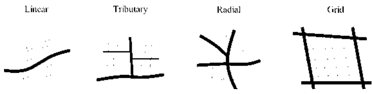
Street Networks Conventional transport network analysis methods use planar representations to reduce a complex transport network into a set of fundamental elements: nodes that represent junctions and links that represent roads (Lowe, 1975). A two dimensional set of systematically organised points and lines like this are referred to as a planar graph. These are the basis upon which various forms of spatial analysis normally proceed (e.g. Bowen, 2012; O’Kelly, 1998). Marshall (2005) identifies four ‘archetypal’ street patterns, the ‘linear’, ‘tributary’, ‘radial’ and ‘grid’ (as shown in Human Aspects of Transportation II (2021)
Figure 1).
Figure 1. Urban street pattern archetypes
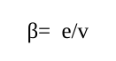
Network diagrams provide a visual representation that, in simple cases, makes it very easy to discern one archetype from another. In more complex real-world networks the visual complexity makes this task difficult to perform reliably and objectively. In these cases it is possible to turn to a number of formal metrics drawn from graph theory. These enable the connectivity of street patterns to be calculated. Three metrics, the ‘Beta Index’, the ‘Gamma Index’ and ‘Network Depth’, are used for this purpose. The Beta Index is a simple equation used to determine the relationship between the total number of links and the total number of nodes in a network and is calculated using the following equation:
Equation reproduced from the original PDF.
Where e = number of links, v = number of nodes and 0.5 < β < (v-1)/2. The Beta Index provides a measure of linkage intensity or “the number of linkages per node” (Lowe, 1975). Beta values generally lie between 0.5 and 3, with networks having values > 1 consisting of nodes within the network having more than one route between them, and the network being considered well connected. Beta values <1 indicate that the network is not as well connected and there being only one route between nodes.
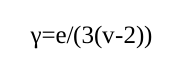
The ‘Gamma Index’ helps to identify “the ratio between the actual and the maximum possible number of links” in the network (Lowe, 1975). This essentially determines whether or not every node is connected by a link and is derived from the following equation:
Equation reproduced from the original PDF.
Where e = number of links, v = number of nodes and 0 < γ < 1. For example, if γ = 0.5 only 50% of the maximum possible number of links in a network are provided and not all of the nodes are fully connected.
The ‘depth’ of a network is a relatively simple concept. In essence, it accounts for the relative distance between the most minor route and the most major route. It establishes the idea of a hierarchy and the different interconnections that exist between levels. For example, minor roads providing access to houses are ‘deep’ whilst major routes are ‘shallow’. Network depth is important if the goal is to impartially compare different street patterns. If one network was to have a depth of four and another a depth of two, the so called deeper network would have more connectivity. This would allow the road user to travel between points in a shorter period of time as there would be more route choice options for a road user to exploit. Different street patterns (with different Beta and Gamma coefficients) can be legitimately compared if the network depth is kept constant.
Abstracting street patterns to the level of planar networks puts them on the same level as communications and other network types, for which there is a rich literature in the fields of graph theory (Harary, 1994), sociometry (Leavitt, 1951; Monge & Contractor, 2003) and complexity (Watts & Strogatz, 1998). We know from this literature that Human Aspects of Transportation II (2021) network type is a strong contingency factor in how they perform (Leavitt, 1951; Pugh et al., 1968; Watts & Strogatz, 1998 etc.). This is in opposition to the tacit theories underlying telematics technologies, which tend to assume that more technology, more route guidance, and more driver knowledge of the wider traffic conditions, the better the network will perform (Nijkamp, Pepping & Banister, 1997). We know from the wider literature on communication networks that this is not necessarily the case. Of course, roads are not communications networks in the way they have been previously studied, so in order to explore the hypothesis that street pattern is an important contingency factor in the benefits to be accrued from telematics technology, we apply instead an agent modelling approach called traffic microsimulation. Microsimulation enables us to create a set of virtual street layouts based on real towns and cities, populate them with virtual traffic having differing levels of route guidance, and observe the outcomes in terms of journey length, duration, cost, and most importantly, carbon emissions. This is an exploratory study which aims to examine the highly systemic nature of traffic and transport, revealing how strategies focused on individual drivers may (or may not) propagate through the system as a whole to give rise to effects that we want and expect.
METHOD
Design The study uses traffic microsimulation to test the interaction between different levels of vehicle telematics and the outcomes achieved within different street patterns. There are four dependent variables: journey duration, journey length, journey cost and carbon output. These dependent variables are contingent upon two independent variables: driver knowledge of the traffic conditions in the network provided by telematics, and street pattern type. Driver knowledge had three levels. 100% telematics represented urban delivery vehicles in which every driver had complete knowledge of the traffic conditions on the network and was required to act upon the guidance given (a ‘best-case’ telematics implementation). 50% telematics represented other non-freight vehicles in the network equipped with telematics/route guidance/sat nav etc. but which, in accordance with the literature, only complied with/took notice of 50% of the information provided. 0% telematics represented vehicles with no route guidance, with the driver having only immediate local knowledge of traffic conditions based on what they can see. Street pattern had four levels: linear, radial, grid and tributary. The street patterns were based on real urban locations, with network depth held constant in order to control for non-systematic biases in connectivity. Network demand was based on real-life traffic count data from the relevant sites.
Real-World Problem As determined in the previous section, there are four common forms of urban transport network layout: linear, radial, grid and tributary. It was necessary to develop microsimulation models which closely reflect the layouts of these urban networks and it was considered important to relate the layouts to real life towns and cities. This gives a more realistic approach and a more credible set of results. The Beta and Gamma coefficients were used to calculate the connectivity of the network archetypes shown in Figure 1 in order to select real-life road networks exhibiting the same properties. This approach allows networks to be categorised by a visual and a statistical approach. The depth of each model was set to three in order to control for the effects of network connectivity.
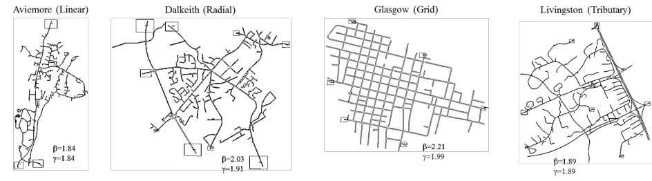
The Linear network required locating a small town in which there is one main road with the town located along its length. A settlement identified as meeting these criteria is Aviemore, a town located in the Scottish Highlands. The Radial network is one that has several roads intersecting or converging at a centre, analogous to the spokes of a bicycle wheel. These features can often be found in a larger town which has formed at a cross roads. These criteria are met by Dalkeith, a town located just to the south of Edinburgh. The Grid network, as its name suggests, is a network with straight roads intersecting other straight roads at right-angles to form a collection of squares or blocks. The characteristics of this network type are found in the center of Glasgow. Finally, the Tributary network is analogous to tributary rivers, with the smaller rivers feeding the bigger rivers. In road networks, it is the small roads that connect to the larger roads with ‘Network Depth 1’ only connecting to ‘Depth 2’ and ‘Depth 2’ only connecting to ‘Depth 3’ and so on. The result of this is that only the shallower roads are busy and the deeper roads are not used as shortcuts. An area meeting the description of a Tributary network is Livingston, a so called ‘new town’ in central Scotland. Planar graphs of these real-life street networks are shown in Figure 2 along with their respective network metrics.
Figure 2. Traffic microsimulation models of Aviemore (tributary), Dalkeith (radial), Glasgow (grid) and
Livingston (tributary).
Beta and Gamma values were calculated for each of the real-life towns to check the extent to which they conform to the linear, radial, grid and tributary archetypes. The real-life networks are considerably larger than the archetypes yet it can be noted how closely the network metrics align. The Beta values for the ‘Linear’ and ‘Aviemore’ networks, for example, are exactly equal as are the Beta values for the ‘Tributary’ and ‘Livingston’ networks. Even where differences do exist (and they are relatively modest) the rank-order of the network types is still preserved.
Development of Network Models Planar graph representations of Aviemore, Dalkeith, Glasgow and Livingston were extracted from ArcGIS (a mapping and spatial analysis software) and imported into S-Paramics (the traffic microsimulation software) in order to create a basic model of each. An attempt was made to ensure that the modelled network was as true to life as possible but some simplifications were required to ensure uniformity. As such, junctions had simple priorities applied with the bigger roads having priority over the smaller roads. Traffic lights were avoided all together. There were also no buses or bus routes applied as not all networks had buses arriving at similar times and some networks had bus lanes whereas others did not. The so-called ‘signpost distance’ refers to the distance ahead of a hazard that the modelled road users become aware of it, and was standardised to 80 m to allow the traffic to use both lanes of the entrances and exits of roundabouts (anomalous behaviour would arise if not). Visibility was also varied. This relates to how far back from the stop-line vehicles begin assessing their gap distance. This ensured vehicles approaching roundabouts continued onto it in situations where nothing was coming and stopped in cases where something was approaching. The distance which meant vehicles followed this rule was found to be 20m. These rules allowed more life-like driver behaviour to be represented and were applied consistently across all the networks in order to isolate the effects of network and vehicle type.
Vehicle Types The principle vehicle-based manipulation was the amount of route guidance provided to drivers, or as modelled, the amount of knowledge drivers had of wider network conditions. The three levels of familiarity were as follows:
Vehicle Type 1 (Urban Delivery Vehicle) - 100% knowledge: drivers have full knowledge of the state of the current road network via telematics and they follow route guidance implicitly.
Vehicle Type 2 (Private Car) - 50% knowledge: implies a vehicle fitted with telematics but one in which the driver chooses to ignore 50% of the network information provided.
Vehicle Type 3 (Private Car) - 0% knowledge: implies a vehicle without telematics, hence the driver has no knowledge of the road network’s state beyond what they can see ahead of them.
The three levels of familiarity were implemented in the microsimulation model by manipulating feedback. Feedback is information supplied to the road user, via telematics, about the current network conditions. Specifically, it lets them know of journey times on all routes so they can decide an optimum route to choose. Feedback is calculated using two aspects, the feedback interval and the feedback factor. The feedback interval refers to how often the information is updated and an interval of two minutes was used (this being a common value in similar models). The feedback factor is concerned with what percentage of delay information is taken from the previous feedback interval and was taken to be 0.5 or 50% as standard. A perturbation level of 5% was applied to all three vehicle types. This helps to account for variability in travel costs, or a driver’s perception of these travel costs. As perturbation increases, the road users’ concentration tends to focus more on reducing journey cost. However, by applying a small percentage it means that road users will continue to focus on reducing journey length and journey duration as the key variants but will also look to reduce their cost simultaneously.
The same mix of traffic was applied to all the networks in order to capture the interaction between ‘normal traffic’ and urban freight delivery vehicles. 50% of the road users in all the network types were ‘Vehicle Type 3’ (0% telematics) with the remaining 50% being split in two; 25% of road users were ‘Vehicle Type 2’ (50% telematics) and 25% of road users being urban delivery vehicles, or ‘Vehicle Type 1’ (100% telematics). The normal traffic (i.e. Vehicle Types 2 and 3) were modelled as medium sized saloon cars, whereas the urban delivery vehicles (i.e. Vehicle Type 1) were modelled as car-based vans. This is a) because larger vehicle types would give unfavourable differential effects on networks that are less suitable for larger vehicles and b) the literature identifies vans as the ‘dominant mode’ in urban contexts (e.g. Cherrett, 2012).
Network Demand The demand profile controls the number of vehicles in the network, the origin and destination of the vehicles, the percentages of vehicle type and the release rate of vehicles into the network. The number of vehicles released from the Origin to the Destination was varied from model to model based on actual traffic count data. The goal was to bring each network to its peak PM traffic flow and hold it there for the duration of the study. To do this, peak PM values from the nearest traffic counter site (Scottish Government, 2012) were used and multiplied by 24. This total value was then split evenly between each of the Origins and Destinations. The release rate of the vehicles over the 24 hour period was constant so that all the vehicles were not released at once and a steady flow was maintained. Each model was then subject to 30 ‘batch runs’ between the network model hours of 1600 and 2000, which was the length of the PM peak flow period. The models had, of course, been established in this peak flow state for many hours previously hence any transient effects of the model being initially loaded with traffic were avoided. These 30 runs allowed a significant amount of data to be obtained on the outcome variables of journey duration, length, cost, carbon output and their contingency on network type.
RESULTS AND DISCUSSION
S-Paramics microsimulation outputs a set of raw data for each individual vehicle as it progresses through the network. The software calculates the position of each individual vehicle every half second and records its co- ordinates against time. This data was passed through an external programme known as ‘AIRE’ which calculates the resulting pollution output of each individual vehicle for a specific year, which was chosen to be 2012. An average value for Carbon Output was obtained for each vehicle type, along with data on journey duration, length and cost. A summary of the results is shown in Table 1, corrected for network size/distance, and collapsing some of the key variables into average speed, cost per km, carbon output in g/Km and total emissions.
Table 1 - Summary of corrected speed, cost and carbon output data
Ignoring the effects of route guidance for a moment, it can be noted that the linear and radial networks are very similar, both being able to support average speeds in the region of 42Km/h, costs per Km of approximately 27 pence, with vehicles on the network each emitting approximately 60g/Km of carbon. The tributary is the same aside from cost, which is the lowest of all the road networks at 15.99 pence/Km. The slowest (33.28Km/h), most expensive (70.53 pence/Km) and carbon intensive (92.77 g/Km) network is the ‘Grid’ but it is within this network that the urban delivery vehicles (with 100% route guidance) performed the best. In this situation telemetry is raising average speeds by 2.9Km/h, reducing costs by a not insignificant 10.47 pence/Km and, most importantly, reducing carbon emissions by 12.21g/Km. The carbon value is of course determined by the physical size of the networks and the journey lengths therein, so in these examples the larger tributary network (i.e. Livingston) has the highest total emissions (3.8 tonnes of carbon per modelled PM peak), however, the network with the shortest average journey lengths (i.e. Glasgow / Grid) has the second worst carbon outputs (2.2 tonnes).
There are smaller differential effects present in the other network types that are also important. Although smaller at the level of individual vehicles, when multiplied by the number of vehicles in the networks (several thousand) and the number of times PM peak hour conditions occur (every weekday evening) these differences begin to magnify significantly. For example, in the tributary network, a per-vehicle difference in carbon emissions of only 0.7 grams as a result of route guidance still multiplies to an additional daily PM peak carbon output of approximately 4.2Kg, or approximately 1 tonne per year. Multiplied again by the number of settlements with tributary street patterns and these initially marginal differences start to accumulate rapidly. With this in mind, the following sections shift the focus from absolute values to relative values in order to discern the direction of these various effects, and what they might mean for an overall telematics strategy.
Route Guidance vs. Journey Duration Urban delivery vehicles (with 100% telematics) operating within linear and tributary road networks are worse off than ‘normal traffic’ with 50% knowledge/acceptance of route guidance information, albeit not as bad as the population of vehicles with no route guidance. Indeed, the results show that the same outcomes on journey duration are achieved at both 100% telematics penetration and approximately 20%, the difference being that the latter is considerably more costly than the former. The trend line obtained for the ‘Radial’ network only slightly differs from the ‘Linear’ and ‘Tributary’ networks in respect of the duration increasing between 50% and 100%, and levelling off thereafter. This shows there is no further benefit of route guidance in this context. The relationship for the ‘Linear’, ‘Radial’ and ‘Tributary’ networks seem to show that there is an optimum level of route guidance. For the optimisation of journey durations a level of knowledge consistent with 100% telematics is not required. This principle does not hold for the ‘Grid’ network. Here the trend line shows increasing benefits as more telematics is provided, reaching a maximum benefit at 100% telematics penetration. The broader principle to be extracted here is that 50% route knowledge is optimum for networks characterised by one or two critical routes between the majority of the origins and destinations. 100% telematics penetration reduces journey durations in networks where there are a large range of routes available to the road user. In this study, urban freight vehicles with 100% route guidance extract maximum journey time benefits in Grid networks.
Route Guidance vs. Journey Length In the linear network, the journey length increases at a slow rate between 0% and 50% route guidance before it increases at a much greater rate between 50% and 100%. This relationship is very different from the Radial and Tributary networks, which both have a long journey length for road users with 0% but falling markedly between 0% and 50% before rising again very steeply between 50% and 100%. As with the results for journey duration, there is an optimum level of route guidance for Radial and Tributary networks (around 50%), with the same network performance achieved at 0% route guidance as achieved at 100%. Urban delivery vehicles with 100% route guidance would see little benefit in these settings. The Grid network differs again. The greater the amount of route guidance the greater the journey length as road users exploit the more numerous opportunities to divert. Taken together, the findings suggest that shorter journey durations are achieved with longer journey lengths. The broader principle to be extracted here is that urban freight vehicles in networks with more than one route between the origin and destination travel a greater distance but in a shorter time.
Route Guidance vs. Journey Cost The Linear network has a more or less direct relationship between route guidance and journey cost (i.e. a straight line). It shows that as route guidance increases from 0% to 100%, the journey cost also increases. Interestingly, in this network type 0% route guidance is the optimum value for cost to be optimised. This is not the case for Radial and Tributary networks. Both of these undergo a reduction in cost between 0% and 50% with an increase then occurring between 50% and 100%. Once again, the optimum level of rote guidance in a Radial or Tributary network is 50%, with further increases not only having a negative effect on journey cost but 100% telematics penetration (as per the urban freight vehicles) yields the same outcome as 0%. The Grid network again performs differently to the other three network types. The relationship is linear (i.e. a straight line) between 0 and 50% route guidance, before tailing off slightly as 100% telematics penetration is reached. What this means is that 100% route guidance is required in Grid networks for meaningful journey cost savings to emerge, 0% for linear networks and 50% for Radial and Tributary networks.
Route Guidance vs. Carbon Emissions The crux of the analysis is to see what effect these contingent values of journey length, duration and cost ultimately have on carbon emissions. The results show the Linear, Radial and Tributary networks all following a similar trend, with carbon emissions decreasing rapidly between 0% and 50% route guidance but with varying levels of diminishing further benefits as route guidance approaches 100%. The Linear and Radial networks level off beyond 50%, suggesting little (if any) further benefits of increasing the amount of route guidance. The results suggest the carbon emissions from the Tributary network worsen with increases beyond 50% route guidance. The ‘Grid’ network is once again quite distinct. It contains a directly proportional relationship between route guidance and carbon emissions, with the maximum value occurring at 0% and the minimum value at 100%. If reducing carbon emissions are the goal of urban freight vehicles then route guidance has the biggest role to play in Grid networks, and apart from Tributary networks, there are some benefits to be extracted before 100% route guidance is achieved.
Optimisation Values Based on the data and relationships obtained from the previous sections, it is possible to create Table 2 to show the potential network performance trade-offs involved in minimising carbon emissions using route guidance technology. A mean level of route guidance (or acceptance thereof) is given, this representing a simple value by which the best compromise of journey duration, length, cost and carbon variables is achieved.
Table 2 – Optimum levels of telematics penetration for journey duration, length, cost and carbon emissions for linear, tributary, radial and grid street patterns
Table 2 shows that, in theory, urban street networks can be designed to be sustainable with the smallest pollution outputs, designed to reduce the journey duration of road users travelling through them, or designed to reduce traveller costs. In practice, however, street networks have evolved and cannot be changed on the scale necessary to optimise these factors. This is where telematics comes in. Telematics interacts with network types to modify their inherent performance but the interaction is not a simple one. It is contingent on the level of telematics information provided to, and accepted by, drivers, combined with the topology of the network itself. Where some networks require varying amounts of route guidance to optimise different aspects of the network, some run at the optimum level for the majority of characteristics under one level of route guidance. This can be seen in Table 2 with the Tributary and Radial networks, which both run at their most efficient levels for all four characteristics with a 50% telematics rate. The table also shows that for a Grid network, 100% route guidance is the optimum value. Linear networks, however, do not reach their optimum level of efficiency for any one level of telematics. Table 2, therefore, becomes a useful tool when attempting to design a telematics strategy in order to modify the inherent characteristics of urban road networks. Stated simply, some levels of driver knowledge of network conditions (provided via telematics) are more optimal than others, and it depends on the street pattern urban road users are operating within.
Fundamental Relationships The results shown and discussed above convey the idea that for each output characteristic (i.e. journey length, cost, duration, carbon emissions) different vehicles perform differently depending on the route guidance provided to drivers. What if a particular urban freight context does not conform to the archetypes presented? In this case it is possible to increase the generalizability of the results with recourse back to the connectivity coefficients discussed earlier. These can be applied to any transport network, of any size or type, in order to reveal its underlying level of connectivity.
Figure 2 – Relationship between the Beta Coefficient (β )and the level of telematics required to optimise journey length, duration, cost and carbon outputs.
A fundamental relationship emerges: as the amount of route guidance increases from 0% to 100% in a road network with Beta (β) ≥ 1.9, Journey Costs, Journey Duration and Carbon Output tend to improve (or at least do not worsen). In networks with β < 1.9 there is no added benefit of providing anything more than 50% route guidance. Figure 2 illustrates the relationship between β and telematics within the range of data observed. Figure 2 represents a simple diagnostic for answering the question ‘what are the benefits of increasing drivers’ knowledge of the wider network conditions, via telematics, in a particular operating environment’.
CONCLUSIONS
Contrary to general belief, this study shows there is a point at which more route guidance does not lead to more efficient urban logistics. Indeed, in many cases the same outcomes can be achieved with 0% route guidance as can be achieved with 100%. Simply introducing an abundance of telematics into an urban freight situation, with planners and company policy enforcing 100% compliance with route guidance, however feasible that may be, will not always result in the outcomes expected. This paper shows that the topography of an urban street layout is an important contingency factor in how and when to deploy this technology.
This is an exploratory study but a number of potentially important implications arise from it. The first relates to previous research showing between 30 and 50% of drivers do not comply with telematics-based route guidance no matter how much of it is provided. As the results show, middle values like these represent an optimum on many outcome variables and street network types. This raises an interesting point. Does this established 30 to 50% driver acceptance of route guidance arise through repeated experience of traffic conditions on a network, the implication being that driver behaviour (and the network itself) are self-organising? If this is the case, then is the imposition of telematics based on a false premise? Does ‘everyone’ in the network need to know ‘everything’? The results of this study would seem to suggest that, for some network types, they do not. If this is the case then the same outcomes could be achieved for considerably less cost.
The second implication relates to the different telematics strategies that urban logistics providers could adopt, and when. Is a costly strategy of providing complete knowledge of the network to drivers, and enforcing compliance with route guidance, optimum in all situations? No. Likewise, is a laissez fair approach to planning and route guidance, based purely on ad-hoc local knowledge brought to situations by individual drivers, optimum? Again, no. Optimisation is contingent upon the topology of the network being travelled upon. There are clearly some situations where it would benefit outcome variables such as carbon emissions to impose compliance with route guidance, and other situations where it would not be appropriate. The results of this paper are helpful in understanding what these relationships might be and what an ‘adaptive telematics’ strategy might look like. It would be a form of route guidance that would be cognitively compatible with drivers. One in which the timing and sequence of route guidance information would be oriented around different outcome variables at different times, but in all cases offering tangible journey based ‘rewards’ for the driver. These rewards would encourage telematics to be used in ways that exceed the current 30-50% acceptance rate where it is beneficial to do so, and as such, to accumulate some significant marginal gains.
ACKNOWLEDGEMENTS
This research was carried out under EPSRC Grant EP/K00915X/1 held jointly by Heriot-Watt University, Edinburgh and the University of Cambridge. This research also benefitted from a collaboration between Heriot- Watt University and SIAS Transport Planners, 37 Manor Place, Edinburgh, [UK]EH3 7EB, the developers of the traffic microsimulation software S-Paramics. Further details available at: www.sias.com.
REFERENCES
Asvin, G. (2008). Fleet telematics: real-time management and planning of commercial vehicle operations. Boston, MA: Springer. Bonsall, P, (1992). The influence of route guidance on route choice in urban networks. Transportation 19, 1-23. Bonsall, P.W. and Palmer, I. (1999). Behavioural response to roadside variable message signs: factors affecting compliance. In:
Emmerick, R and Nijkampt, P. (eds). Behavioural and Network Impacts of Driver Information Systems. Farnham: Ashgate. Bowen, J. T. (2012). A spatial analysis of FedEx and UPS: hubs, spokes, and network structure. Journal of Transport Geography, 24, 419-431. Brindle, R. E. (1996). Urban Road Classification and Local Street Function. Australian Road Research Board. Cherrett, T., Allen, J., McLeod, F., Maynard, S., Hickford, A. & Browne, M. (2012). Understanding urban freight activity – key
issues for freight planning. Journal of Transport Geography, 24, 22-32. Chorus et al. (2006). Use and effects of Advanced Traveller Information Services (ATIS): A review of the literature. Transport Reviews, 26(2), 127-149. Dutton, G. (2011). Fleet management’s magic box. World Trade, 24(2), 38-44. Giannopoulos, G. A. (1996). Implications of European transport telematics an advanced logistics and distribution. Transport
Logistics, 1(1), 31-49. Harary, F. (1994). Graph Theory. Reading, MA: Addison-Wesley. Hesse, M. & Rodrigue, J. P. (2004). The transport geography of logistics and freight distribution. Journal of Transport Geography, 12(3), 171-184. Karl, C. A. and Bechervaise, N. E. (2003). The learning driver: issues for provision of traveller information services. 10th World
Congress and Exhibition on Intelligent Transport Systems and Services, Madrid. Leavitt, H. J. (1951). Some effects of certain communication patterns on group performance. Journal of Abnormal and Social Psychology, 46, 38-50. Lowe, J. C. (1975). The geography of movement. Boston: Houghton Mifflin. Lyons, G.,Avineri, E. and Farag, S. (2008). Assessing the demand for travel information: do we really want to know? Proc.
European Transport Conference, Noordwijkerhout, Netherlands, October. Marshall, S. (2005). Streets and Patterns. Oxon and New York: Spon Press. Monge, P. R. & Contractor, N. S (2003). Theories of communication networks. New York: Oxford University Press. Nijkamp, P., Pepping, G. & Banister, D. (1997). Telematics and transport behaviour. Berlin Springer-Verlag. O’Kelly, M. E. (1998). A geographer’s analysis of hub-and-spoke networks. Journal of Transport Geography, 6(3), 171-186. Pugh, D. S., Hickson, D. J., Hinings, C. R. & Turner, C. (1968). Dimensions of organisation structure. Administrative Science Quarterly, 13(1), 65-105. Ratan, P. (2013). Telematics: an emerging solution to streamline logistics. Cargo Talk, 13(5), 20-24. Reggiani, A., Lampugnani, G., Nijkamp, P. & Pepping, G. (1995). Towards a typology of European inter-urban transport
corridors for advanced transport telematics applications. Journal of Transport Geography, 3(1), 53-67. Thomson, J. M. (1977). Great Cities and Their Traffic. London: Victor Gollancz Ltd. Watts, D. J. & Strogatz, S. H. (1998). Collective dynamics of ‘small-world’ networks. Nature, 393(4), 440-442.
LISTED IN THE AHFE DIGITAL BOOKSTORE CATALOGUE
Explore the complete digital volume
Advances in Human Aspects of Transportation: Part II
Read this individual research paper free through the original publisher, or explore the full digital proceedings book.
ISBN 978-1-4951-2098-5
Explore this ISBN in the AHFE Bookstore ↗Listed in the July 2026 bookstore catalogue; search by ISBN to confirm current availability · Digital book purchase optional