Capt. Joseph K. Maddux (2019). Applying Factor Analysis to Population Surveys in Afghanistan to Facilitate Improved Decision Making. In: Advances in Cross-Cultural Decision Making. AHFE Open Access, vol. 6. https://doi.org/10.54941/ahfe100199
As the U.S. Military’s involvement in Afghanistan has changed from a traditional kinetic fight to counter-insurgency to nation building, so too has our need to understand the population which we seek to assist. Multiple agencies have taken on the task of surveying Afghans at the national, provincial and district levels. Conducting these surveys carries great risk due to the presence of Taliban fighters and terrorist safe havens strewn throughout the country. While conducting the surveys has its share of obstacles, properly interpreting the results carry its own unique set of challenges. We use three surveys that have been mainstays as sources of information for the U.S. Military and other nations to understand popular perceptions. Using Factor Analysis on these three surveys collected over the last 3-5 years allows us to analyze all questions and responses in the surveys by identifying the most relevant data analytically vice a subjective analyst or commander deciding what is most important. We do so by using a methodology that establishes quality, analytically derived indicators (groups of survey questions) by using these three survey instruments collected throughout Afghanistan. We generate indicators from survey data using Factor Analysis then assess them by using nonparametric statistics techniques to detect spatial and temporal changes throughout the country. The final result is a full analytics suite that provides perspective to an analyst regarding indicator change across the country over time. Further, we improve the commander’s ability to allocate scarce resources to particular districts and provinces which need the most attention.
The United States Military has been conducting Operation Enduring Freedom in Afghanistan at various commitment levels since 2001. While the initial U.S. interests were to eliminate Osama Bin Laden and his Al-Qaeda forces, efforts shifted to more of a counter-insurgency (COIN) engagement. In order to victor in a counter-insurgency environment, it is typically important to gain the trust and confidence of the local populace by ensuring that they are being treated fairly. On one hand, it is fairly easy to assess our efforts to repel and defeat the enemy. We use intelligence reports to understand where the enemy is and what their plans are and we conduct operations to destroy their resources, deny them access to population centers, crush their will to fight, or dismantle their leadership network to cause disarray in their efforts. The usual device for assessing our actions is to gauge our performance against a set of Measures of Effectiveness (MOE) (United States, 2011). These MOEs are set in place before operations are conducted and our progression towards them is gauged during and after the operation. Meeting all MOEs is not necessarily required to call a mission a success, but having a plan in place to judge where we were against where we are allows us to understand whether our actions were successful. Understanding how much, or even if, we are changing the populations attitudes is much harder. Does the population support the fact that we are in their country, sometimes fighting their husbands, brothers and sons, sometimes destroying their infrastructure, or interrupting their way of life for what we promise to be a better, more fulfilling lifestyle? This type of question is at the forefront within the higher levels of the International Security Assistance Force (ISAF).
One way that we have tried to understand the people is by using survey data. Surveys are a proven, useful way to gauge public perception. They are used every day for all types of reasons from making predictions about an upcoming election to deciding whether a company should introduce a new product to market. Surveys are conducted in Afghanistan for mainly one reason. That reason is to answer the question: Are we winning the hearts and minds of the Afghans? Typically a survey will ask a series of questions that are demographic in nature, i.e. how old are you, are you employed, where do you live and so on. The meat of the questions, though, lies in the perception questions; i.e. how has your district government performed over the last six months or do you feel that the removal of the Taliban is good for the country? In some surveys, hundreds of these perception questions are asked all in an effort to answer one real question. We analyze these hundreds of questions asked to thousands of respondents to gauge our progression towards the MOE of winning hearts and minds of Afghan locals. Unfortunately when analysts do this type of work what they tend to do is pore over the list of questions and select some subset of questions that they feel will provide the best gauge of the MOE. This method of selection is a form of bias that the analyst is putting on their own analysis whether intended or not. Using a western mindset to decide what is important to Afghans is not a wise choice if the chooser does not have an intense understanding of the culture and history of Afghanistan which most analysts do not possess. Conducting these surveys is extremely expensive both in terms of money and man-hours and sometimes quite dangerous, especially in a place like Afghanistan. Why then would we spend so much time and money asking thousands of people hundreds of questions then only analyze one or two of them as a basis for our decisions?
In this research I intend to show that using Factor Analysis on these perception questions is a better choice. By using Factor Analysis we can use all of the perception questions in the survey and let the survey tell us which ones are important. Factor Analysis will group the questions of a survey in to categories known as Factors. We find that these Factors are groups of similarly-themed questions. Each question in the group has a correlation coefficient depicting how well a particular question correlates to the group. These values can also be thought of as weights of each question within the Factor. The questions serve as an observed variable (i.e. a question that was asked directly) and the Factors serve as unobserved variables (i.e. topics that were never brought up during the interview). The interesting thing about Factor Analysis is that we can now make judgments about how a topic has changed over time and where it has changed over time (through using the demographic data) without ever having to ask about the topic directly. In this research we use these Factors as indicators of progression toward an MOE. We generate indicators (factors) from survey data using Factor Analysis and assess them by using nonparametric statistics techniques to detect spatial and temporal changes throughout the country. Then, we use the concept of Exploratory Data Analysis (EDA) by displaying spatial and temporal changes that have occurred as part of an analytics suite to build a better knowledge base of popular perceptions. While EDA will not only give us a better understanding of if, and where, positive changes are happening, it will also give us the opportunity to further explore why positive changes are or are not happening by digging deeper into a particular area of interest to improve the situation.
BACKGROUND OF AFGHANISTAN SURVEY INSTRUMENTS History
Once the focus of Operation Enduring Freedom shifted from a traditional, kinetic fight to counter-insurgency so did the emphasis on improving infrastructure, enhancing youth education, increased employment, the provision of healthcare for the populace along with better governance and development. Efforts were introduced to gauge the perceptions of the local population through surveys. Each of the surveys used in this research carry a slightly different purpose and scope. The surveys started as early as 2008 and have all continued in varying degrees of granularity and recurrence (every 2-4 months) since then. Afghanistan’s administrative borders follow a model of Country, Province, District, and City similar to the way the United States follows a Country, State, County, City model. Afghanistan’s Ministry of Interior officially recognizes 34 Provinces and 398 districts (CIA, 2014). The level of granularity to make judgments on a particular geographic level depends largely on the survey’s sample size in that geographic level. Due to proprietary and classification reasons, these surveys will be referred to as Surveys A, B and C throughout this report. Each of these surveys is described in more detail below.
Survey A The first iteration (each iteration is known as a Wave) of Survey A was conducted in the summer of 2008. This survey is conducted on a roughly quarterly basis (i.e. every 2-3 months) at a nationwide level. It can be parsed to the Provincial level or higher due to its sample size in each province. As with the other surveys in this research, even though each province and district has representation, not all areas of a district are reachable due to various reasons, chiefly security of the area. Each wave of this survey has approximately 12,000 respondents from all 34 provinces and all 398 districts. The pros of Survey A include the national scope and its longevity; 22 Waves of this survey have been conducted to date. The con of the survey is simply the degree to which the questions in the survey have changed over time. This is to be expected sometimes since the ideas and topics researchers are trying to understand will change just as the level of stability in the country has changed.
Key areas of discussion within Survey A include (in no particular order):
Security and safety of roads and community
The performance of the Government of the Islamic Republic of Afghanistan (GIRoA), the Provincial Governor (PG) and the District Governor (DG)
The corruption of various government officials
Family’s economic state, their satisfaction with healthcare and education, and their perceived future outlook of the same
The Taliban’s ability and propensity to rejoin the Afghanistan society
Satisfaction with infrastructure such as roads, electricity and water
Propensity for crimes and violence in the community
The ability of GIRoA and the Afghan National Army (ANA) to succeed without ISAF Survey B
The first Wave of Survey B was conducted in the spring of 2010 and has been conducted on a roughly quarterly basis at a nationwide level. It can be parsed to the provincial level or higher due to its sample size in each province. Similar to Survey A not all areas are represented in Survey B for similar reasons; representation exists from only 26 provinces and 137 districts. 14 Waves of Survey B have been conducted with approximately 7,000 respondents per Wave; the most recent Wave taking place in October 2013. This survey has had a more consistent set of questions over its duration with only minimal change as compared to Survey A.
Key areas of discussion within Survey B include (in no particular order):
The performance of the PG, ANA, and Afghan National Police (ANP)
Satisfaction with infrastructure such as roads, electricity and water
Abuse of power and corruption amongst various government officials
Family’s current quality of life and its future outlook Survey C
Survey C is the survey that is most familiar to the author and is quite different than the previous two surveys in many ways and similar in others. Survey C is only focused on one province of Afghanistan, Helmand Province. This granularity of the survey is down to the district level since the sample size of each district is large enough to allow for statistically significant judgments on of each district. Survey C was initially conducted in October 2010 and has been conducted on a roughly quarterly (2-4 months) basis ever since. Each wave of this survey has approximately 4,000 respondents that are fairly evenly distributed amongst nine of Helmand’s 12 districts.
Key areas of discussion within Survey C include (in no particular order):
The performance of the DG in governance, infrastructure and employment opportunities, etc.
General satisfaction with infrastructure, education and health services
Performance of ANA and ANP
Ability of various levels of leadership to solve disputes fairly, address corruption and provide security to their districts
Expectations of future infrastructure, education and health services
Fairness of district, provincial and national level judicial system
METHODOLOGY
Question Selection and Recoding In order to conduct Factor Analysis we must have a complete data set to work with where each respondent has answered each question. A single missing answer to a question will not allow the mathematics of Factor Analysis to work. The first step in doing this is to determine which questions are the mainstays of the survey we are working with; we’ll refer to these questions as Enduring Questions. In order to compare waves of the survey over time each question must be asked each time. This is almost never the case because situations and interests eventually change over time. Determining the Enduring Questions is typically a labor intensive, time consuming process when starting out; one question not asked in any wave of the survey means that question in all other waves must be dismissed. Unfortunately by doing this we will be losing some of the data but we still have a high number of questions in each of our three surveys to work with; Survey A has 67 Enduring Questions, Survey B has 50 Enduring Questions and Survey C has 91 Enduring Questions.
Once we have our Enduring Questions we must carefully recode the answers numerically. Each of our Enduring Questions requires a three or five-point Likert Scale response. For example a five-point Likert Scale response might look something like “Strongly Agree”, “Somewhat Agree”, “Neither Agree nor Disagree”, “Somewhat Disagree” or “Strongly Disagree” while a three-point Likert Scale response might be “Yes”, “Neither” or “No”. Note that each of these examples has a neutral point and an equal number of positive and negative possibilities as options. For this research we use a numeric recoding scheme of 2 for most positive, 1 for the slightly positive, 0 for neutral, -1 for slightly negative and -2 for most negative for the five-point Likert Scale and a similar 2, 0 or -2 structure for three- point Likert Scale responses. Also, note that I used the words positive and negative instead of agree and disagree. This is due to the nature of question. For example, a question might be asked “Do you support the idea of the Taliban returning to power in Afghanistan?” From ISAFs perspective, a response of “Strongly Agree” would be negative. Conversely a response of “Strongly Agree” to the question “Do you support ISAFs role in reconstruction of your area?” would be seen as a positive to ISAF personnel.
Imputation of Missing Data Next we must deal with those respondents who simply did not answer the question for any number of reasons. Initially these answers are not given a numeric value and are simply recoded as “NA”. But, as stated earlier, these NAs will not allow the mathematics of Factor Analysis to work. One approach to resolving NAs is to perform casewise deletion. For our analysis of survey data, this means that if a respondent has an NA for just one of the Enduring Questions then all of his/her data would be removed from the data set as if the interview never happened. If we used this casewise deletion approach we would be doing a great disservice to ourselves by losing a plethora of information. In order to save this data we can impute the missing values. Imputing the missing values means that we substitute an NA with some other value of -2, -1, 0, 1, or 2. We have to be careful here not to impute “too much” missing data. Unfortunately, there is no good metric that indicates that too much data is missing to use imputation (Stuart, 2010). For this research, we conclude that if a question has less than 20% of the responses missing we allow imputation of the missing values. Because of the measures already discussed in the previous section (i.e. the careful selection of Enduring Questions), none of our Enduring Questions violate this criterion. One way to approach imputation would be to randomly choose the value; this approach is a poor choice because we would simply be guessing. Another approach is to take the mean of the non-missing responses and substitute that value as the response. We could even use the median of smaller subsets of demographic data such as the district the respondent is from or their religion to try to find a more likely response from a person of similar background. But instead we will use a process known as Hot Deck Imputation (HDI). HDI finds a value for the missing value by comparing demographic data of the respondent whose value is missing to demographic data of respondents who answered the particular question.
The initial step of HDI is to make a subset of the data into a “donor class;” for this analysis the donor class for all Waves comes from the district column of the demographic data. Within each district subset, the data is split into two further subsets of “donor” and “receiver.” The receiver subset consists of data where responses are missing for a particular question and the donor subset contains data where all responses have recoded, numeric values. We choose the donor that is most like the receiver based on the receivers’ religion and tribal affiliation. As an example of imputation, say there is only a single donor who has matching demographic data to the receiver. In this case we would use the donor’s recoded response as the value for the receiver’s response. If there are multiple donors whose demographic data is an exact match to the receiver then one of the donors is picked at random and their recoded response is used as a replacement value for the receiver. If there is no exact matching donor then we look for donors that are closest to matching the receivers’ demographics. From this list the same rule applies amongst ties here as it did in the exact matching cases. The HDI process is done for all waves of data as necessary in order to produce complete numerically recoded sets of data. We are now able to use Factor Analysis on our survey data.
Factor Analysis
At its core Factor Analysis serves as a data reduction technique (Garrett-Mayer, 2006). Its use with survey data is ideal because we are typically dealing with a large number of variables (i.e. the questions asked in the survey) and we would like to be able to pare this data set down to some smaller number of variables without losing any of the surveys intrinsic value. Factor Analysis not only does this for us but it also provides us with a correlation coefficient (r), also known as a Factor Loading, that indicates how well each question correlates to the derived factor; -1 ≤ r ≤ 1. These correlation coefficients serve as explanations of variance of each question within the factor and can be used later as weights. Factor Analysis helps to eliminate correlation between Factors while increasing correlation within Factors (Garrett-Mayer, 2010). In short, Factor Analysis provides us with groups of questions that are similar in nature and allows us to work with a smaller set of correlated variables (questions). In the end we have our observed variables, the questions and a new set of unobserved variables, the factors. While we could take the time to look over the questions and group these questions together manually, we would essentially be doing the same thing warned against in the introduction; using a western mindset to decide what is best for Afghans. Additionally, we would be, unintentionally or not, giving each question the same weight of 1. By using Factor Analysis we are able to analytically derive a set of correlated questions, called factors or indicators, and use these indicators as our basis for measuring if and how situations have changed across a province or district.
For this research we use the latest wave of each survey to conduct Factor Analysis which allows us to establish a baseline for each survey to make comparisons from. As a result of using Factor Analysis on the three surveys in this research we reduce our data sets as follows: Survey A is reduced from 67 observed variables to 13 unobserved variables, Survey B from 50 observed to seven unobserved, and Survey C from 94 to 22. For our purposes, we keep only those questions that have a Factor Loading of 0.4 or higher and -0.4 or lower and set the loadings of all other questions to 0 (Example in Table 4). Each factor consists of at least two and up to as many as 12 observed variables.
Results of Factor Analysis Survey A
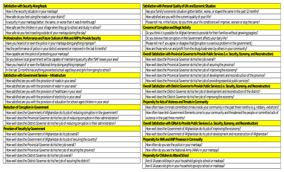
The 13 factors produced by Factor Analysis on Survey A can be viewed in Table 7 of the Appendix. Generally speaking the topics covered by the factors are the satisfaction and performance of various government entities in the areas of security, governance, provision of infrastructure, employment opportunities, and education for children. Two factors in particular are worthy of discussion here and they both deal with corruption. Corruption is very much common place in Afghanistan. For example, anecdotal stories suggest that if a District Police Chief does not keep at least some portion of his policemen’s salary for himself then something must be wrong. I point this out because this type of context is important to understanding corruption in Afghanistan. One of the factors in particular has three questions in it and individually they ask how well GIRoA, the Provincial Governor and the District Governor reduce corruption in their respective governments. The other factor has four questions that more generally cover corruption by asking how serious of a problem corruption is, if it is a serious problem in the government and how those who conduct illicit activity are seen in the community. For U.S. citizens, any level of corruption would call for outrage by the public. In Afghanistan, it is the norm. Later in this research we will discuss various metrics to gauge how this factor has changed over time. We must keep in mind that what we think of as an acceptable level of corruption is much different than what our survey respondents think.
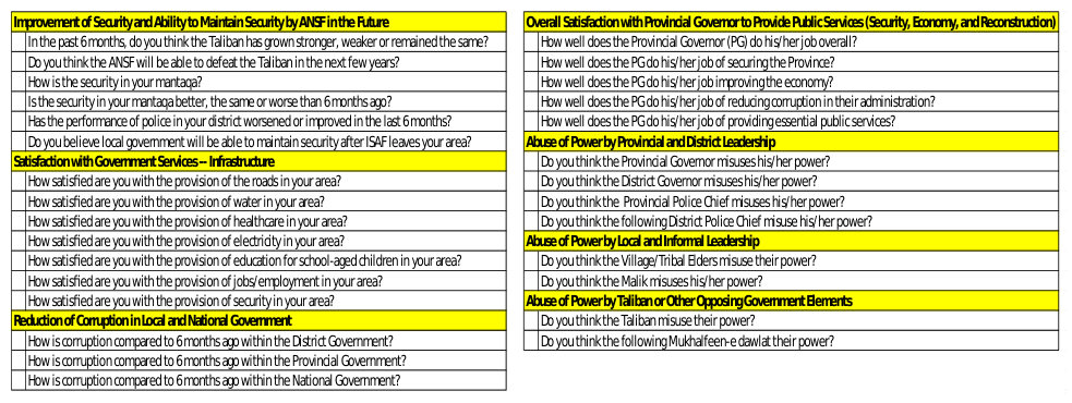
Survey B The seven factors produced by Factor Analysis on Survey B can be viewed in Table 8 of the Appendix. A few of the factors produced for Survey B are similar to those in Survey A in that the questions in the factor deal with reduction of corruption and the satisfaction with governments provision of infrastructure, public services, and security. Two types of factors are worthy of discussion here for Survey B. The first is made up of six questions having to do with the improvement of the Afghanistan National Security Force (ANSF) in providing security and their ability to do so in the future without ISAFs assistance. ANSFs ability to maintain security gains post ISAFs departure is one of the key concerns of the entire operation. Regardless of their actual ability, which will not be truly known for years, we can now gauge the popular perception of this topic. The other factors have to do with abuses of power not only by different levels of leadership, but the Taliban as well. While abuse of power is similar to corruption, it is in fact different. Not only can we gain better understanding of the popular perception of this topic, we can do it at three different levels of leadership. These factors can help us understand these abuses at the formal level of leadership (Provincial and District government) the informal level (the Tribal Elders and the Maliks) and the enemy’s leadership (the Taliban).
Survey C
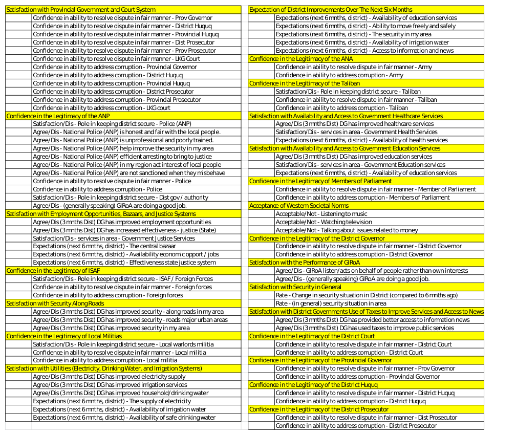
The 22 factors produced by Factor Analysis on Survey C can be viewed in Table 9 of the Appendix. The first and most obvious observation of the results is there are quite a few more factors here than in the other surveys. The second notable observation is that this survey allows forces or other responsible parties to gain a much deeper understanding of Helmand Province in particular. While the general nature of the questions making up each factor is not much different than those in the other surveys, their level of detail and specificity to a particular group is quite valuable. For example, several separate factors use questions that specifically discuss the Afghan National Police, Afghan National Army, ISAF, the Taliban, GIRoA in general, members of Afghanistan’s Parliament, Provincial Government, District Governments, and so on. Other factor topics which are different than our other two surveys include local militias, fair use of taxes, and acceptance of western societal norms. The Factor Analysis results for this survey allow an analyst to gain a much more specific perspective of this province by covering various areas of concern. This type of analysis could not truly be conducted on our other surveys due to their broad range of topics.
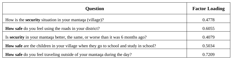
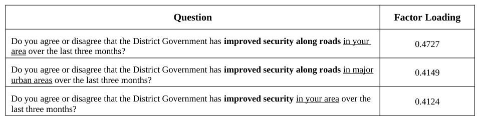
Deriving Indicators from Factors The Factors that we derive are simply labeled initially as Factor 1, Factor 2, etc. Since our desired end state is look at progression towards a particular MOE we will give each factor a more descriptive name. For example, if we look at a selection of Factor Analysis results from Surveys A (Table 1) and C (Table 2) we can see the thought process on naming the indicators and how there are sometimes similarities between the different surveys.
Table 1. Factor 4 as derived by Factor Analysis on Survey A.Table 2. Factor 5 as derived by Factor Analysis on Survey C.
The results displayed in Tables 1 and 2 from Surveys A and C, respectively, carry a similar theme. Namely, each question asks something about security in a particular area. Due to the fact that the security theme, along with safety, persists throughout the questions in Table 1, we give this factor a more descriptive name, “Satisfaction with Security and Safety in Local Area”, and refer to it as an indicator from here on. Similarly, in Table 2, the security theme appears again, this time with more of a focus on roads. In this case we name the indicator “Satisfaction with Security along Roads.” While a different author may come up with a slightly different name for the indicator, the theme of the indicator would have to remain the same. The exact name of the indicator is not important; however, what is important is that we now have an analytically derived indicator that we can measure against. Each question asked carries a particular weight, the Factor Loading, which will be used in the next step to make these comparisons.
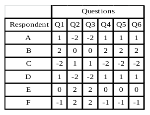
Perhaps the most important takeaway from this is that no one person chose this grouping of questions. In essence, the group of respondents as a whole decided that the topics of these questions were important enough that, individually, each respondent tended to answer each of the set of questions in a similar manner. That last sentence often causes confusion. It’s not that everyone in the survey answered, or even tended to answer, all questions of the indicator the same way. It’s that each person, individually, tended to answer each of the indicators’ questions similarly. A notional example of how one case of Factor Analysis might work on a dummy data set is helpful to understand this concept better. Table 3 shows a dummy data set with six questions and six respondents. Each answer is recoded similarly to the structure we are using in this research. At first glance, an obvious pattern may not be noticeable. But a closer, more studious inspection reveals something about two groups of the six questions. Each respondent tended to answer questions 1, 4, 5 and 6 the same way. In fact, in this extreme example they each answered them exactly the same way. Similarly, they each answered questions 2 and 3 the same way. While between respondents the answers to questions 2 and 3 are sometimes different and on each end of the integer spectrum of -2 to 2, the respondent that answered Q2 with a particular value always answered Q3 with that same value. Even if the reader was able to quickly notice the pattern immediately within this dummy data set, it would be impossible to expect anyone to notice these patterns on data sets of 67 questions and upwards of 12,000 respondents, like Survey A, or 93 questions and 4000 respondents, as is the case in Survey C.
Table 3. Example of Matrix used for Factor Analysis Table 4. Example of Factor Analysis output All of the indicators (44 in total amongst the three surveys) are named in the same manner as described above. A full list of each surveys indicator, its questions, and the factor loadings can be found in Appendix A.
Calculating Respondent Indicator Scores After recoding all of our survey responses to numeric values and conducting Factor Analysis on the last wave of each of our surveys, we want to calculate an indicator value for each respondent in each survey. We’ll refer to this value as the Score. To do these calculations we will be using two matrices. The first matrix, A, is the recoded survey responses. It is an n X m matrix where n = the number of respondents in the survey wave and m = the number of Enduring Questions in the survey. The second matrix, B, is the survey’s Factor Analysis output. This matrix is an m X p matrix where m is, as in A, the number of Enduring Questions in the survey and p is the number of factors that were generated from Factor Analysis. To calculate each Score, we use simple matrix multiplication on our two matrices as described in Equation 1. The output of Equation 1 for each survey wave will be an n X p matrix where n and p are as described previously.
Equation reproduced from the original PDF.
Equation 1. Matrix Multiplication
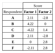
The results of Equation 1 on Tables 3 and 4 can be seen in Table 5. We can see in Table 5 that each respondent in our survey now has a Score for each indicator. A layman’s example of the math follows: for respondent A in Table 3 we would take each of his recoded answers and multiply them by the corresponding Factor Loading and sum those products. So we find the sum of (1 x .53) + (-2 x 0) + (-2 x 0) + (1 x .47) + (1 x .49) + (1 x .62) equals 2.11. This means respondent A’s Score for Factor 1 for our dummy survey is 2.11. We use this process for each respondent in each wave of each of our actual surveys to calculate all factor Scores for all survey respondents. Throughout this process we have saved the respondents’ home district or province to represent changes geographically which will be discussed later.
Table 5. Respondent Scores
Measuring Change of Indicators Spatially and Temporally
For this research, we want to know if change has occurred for a particular indicator from one wave of a survey to the next for each surveyed province or district of Afghanistan. Surveys A and B will show provincial level change while Survey C will show district level change. In order to do this we’ll use the Mann-Whitney test to compare the Scores of one wave of a survey to the Scores of another wave of the same survey and determine if the Scores tend to be equal between the two survey waves or larger in one wave than the other. The Mann-Whitney test is the nonparametric equivalent to the two-sample t-test that is used to compare the means of two data sets and assumes the means are normally distributed. One key difference between the Mann-Whitney test and the two-sample t-test is that the t-test is used to determine if the means of two sets of data are equivalent while the Mann-Whitney test is used to determine if one set of data tends to have larger values (Scores) than the other regardless of the mean of each data set. As such, the Mann- Whitney test is robust to the influences of outliers.
To conduct the Mann-Whitney test we will use geographic subsets of each survey wave. Surveys A and B will be parsed in to subsets of each province while Survey C will be parsed in to subsets by district. For simplicity sake, we’ll refer to provinces or districts as regions. Our hypotheses to be tested are formally stated below where X is the set of Scores from a particular region in one wave of a survey and Y is the set of Scores from the same region in some later wave of the same survey: H0: P (X > Y) = P (X < Y) H1: P (X > Y) ≠ P (X < Y) A less formal statement of the hypotheses is:
H0: The probability that an X observation exceeds a Y observation is 0.5 H1: The probability that an X observation exceeds a Y observation is not 0.5 Score Source Rank 2.2 From Wave 1.5 2.2 From Wave 1.5 2.3 From Wave 4 2.3 From Wave 4 2.2 From Wave 4 2.4 To Wave 7 2.4 To Wave 7 2.4 To Wave 7 2.5 To Wave 9.5 2.5 To Wave 9.5 3.8 To Wave 11 5.8 From Wave 12 Table 6. Example of Rankings To conduct the test we let n equal the number of respondents in the wave we are measuring from, we’ll call it the “From Wave,” and let m equal the number of respondents in the wave we are measuring to, the “To Wave” and N = n + m (these variables will be used later in this section). We then create a table with N rows and 3 columns. Column 1 is the indicator Score, Column two (“Source”) is used to indicate which sample the Score comes from (i.e., “From Wave” or “To Wave”), and the third column indicates the rank of the Score. We then sort the table by Score from lowest to highest. In the case of ties amongst Scores, of which there are many due to the nature of our data, we average the ranks of each of the ties and each tie score receives the same ranking. Table 6 shows the output of these calculations for a hypothetical example. We then calculate a test statistic, T, which will determine any statistical significance of difference between the two waves. The calculation of T is quite simple as shown in Equation 2. It is simply a summation of the ranks of each Score in our From Wave.
Equation available in the original PDF paper.
Equation 2. Test Statistic for Mann-Whitney
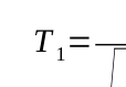
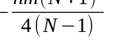
Unfortunately, as mentioned before, there are a high number of tied ranks. Even in the small example above ten of the 12 Scores are tied with at least one other Score. Due to this high number of ties in our survey datas’ Scores we must “subtract the mean number of observations in each data set from T and divide by the standard deviation”
N 2refers to the sum of Ri (Conover, 1999) to get a new test statistic known as T1 (Equation 3). In this equation, ∑ i=1
squares of all N ranks or average ranks actually used in both samples” (Conover, 1999).
T−n N +1
2
Equation reproduced from the original PDF.
2−nm(N+1) 2
Ri
Equation available in the original PDF paper.
Equation reproduced from the original PDF.
√ Equation 3. Test Statistic for Mann-Whitney with Ties Amongst Ranks
Once the T1 Test Statistic is derived we use this to find a p-value. This p-value will tell us, at a given confidence level, whether to accept or reject the null hypothesis; for this research we use a 95 % confidence level (α = 0.05) for each hypothesis test. If the p-value tells us to accept the null hypothesis then we know that there has not been a statistically significant change of the indicator from one wave to the next. However, if the p-value tells us to reject the null hypothesis then we only know that there is a statistically significant difference between the two waves but we don’t know whether the change is higher or lower (i.e. better or worse). To fix this we create a function in R which, instead of requiring the output of a p-value, requires the output to be a -1 if the change is negative, a 1 if the change is positive, or a 0 if there is no change. In order to do this we use the same T 1 test statistic that we calculated above and return a -1 if T1 is in the upper tail, a 1 if it is in the lower tail, or a 0 otherwise.
As an example of this, we calculate Equations 2 and 3 using the data in Table 6. Here T = 27 and T1 = -1.956. This T1 value would tell us to reject H0 with α = 0.05. Rejecting H0 is equivalent to saying there is a statistically significant difference between the two data sets and the value of T1 tells us that, in this case, the Scores in the To Wave tend to be larger than those in the From Wave. In fact, we would further state that there has been a positive change for this indicator. We use this particular hypothetical example to point out the value of using this methodology vice relying on comparing the means of two sets of numbers. The mean of our From Wave Scores is 2.85 while the mean of our To Wave Scores is 2.67. This illustrates the virtue of using the Mann-Whitney test to assess trends. While the mean of the population’s Scores would falsely lead us to believe the population’s Scores trended down from the From Wave to the To Wave, the Mann-Whitney test concludes the To Wave Scores tended to be larger than the From Wave Scores in our example. It is clear by inspection that even with the presence of an outlier from the From Wave, the To Wave Scores in Table 5 tended to be higher than those of From Wave.
DISPLAYING SPATIO-TEMPORAL INDICATOR CHANGE BY SURVEY The statistical significance of change is an important first step in understanding what is happening in our area of interest. Relaying that information to decision makers is perhaps the most challenging aspect. To accomplish this, we will use one of the most common, readily available pieces of software; Microsoft Excel®. Using Excel, we have created an analytics suite, dubbed MICh (Measure of Indicator Change), and designed it to be user friendly and only in need of minor explanation to a first time user. We’ll use the MICh analytics to show three separate metrics of each indicator within the spreadsheet application; the change of the indicator across waves as derived from our Mann-Whitney test, the mean of the indicator in each wave by region, and the proportion of support for each indicator over the duration of the survey by region. Due to constraints we will only show examples from Survey C.
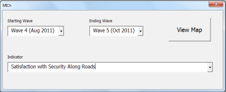
Figure 1. Wave and Indicator Choice Form
MICh uses the indicator Scores and the 1, 0, and -1 codes indicating positive, neutral, or negative change as the basis of its analytics suite. A form in Excel allows the user three options: First, which wave they would like to measure from; our From Wave, Second, the wave they would like to measure to; our To Wave, and lastly, an option to choose one of the indicators. In Figure 1 we see the default options for Survey C where clicking the “View Map” radio button would show the user the three metrics for the “Satisfaction with Security Along Roads” indicator. To choose different waves or a different indicator, the user selects from the dropdown box. Upon clicking View Map the user is presented with a display of our three metrics.
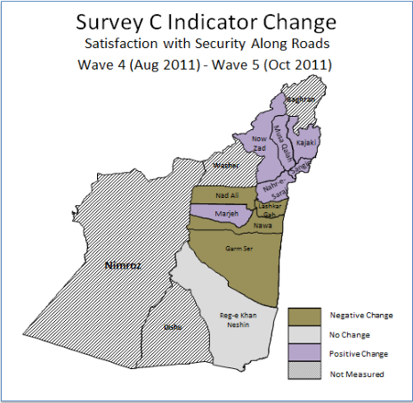
On the map displayed in Figure 2 we see an area of Afghanistan that was commanded and controlled by ISAFs Regional Command Southwest (RC (SW)). The area actually covered two provinces even though Survey C only polled respondents in one, Helmand. Also we see each district of Helmand Province. Three of the Helmand districts are “greyed out”, this indicates that our surveys did not poll any respondents from these districts and therefore they receive a rating of “Not Measured.” Next we see six districts with a purple coloring. Purple indicates a positive change for the indicator. We see that the Reg-e Khan Neshin District is grey; this indicates that there was no statistically significant change here. Lastly we see four districts in brown; this indicates that there was a negative change for the indicator in each of these four districts. What we have shown here is simply whether there has been a change or not, and if so in which direction, but this map alone does not necessarily afford a clear idea of how the general sentiment is to this indicators topic. In other words, we know that our northern districts are more satisfied with the security along the roads in Wave 5 than they were in Wave 4, but we don’t know where, on any type of scale, the actual sentiment lies. To help answer that question we look at Figure 3 which is simultaneously displayed on the screen to the user.
Figure 2. Map of Statistically Significant Change
Figure 3 displays a color coded chart that ranges from red to green for each of our measured districts. A red cell indicates the sentiment of the indicator (during the time period of the surveys wave) to be most unfavorable, green indicates most favorable and yellow indicates neutrality. Rather than simply using the three colors, we use a gradient scale to give us all possible color indications from red to yellow to green. The color of each cell represents the mean Score of the indicator for each district in the province. The extremes of these Scores are set by multiplying -2 by each factor loading for the indicator to get the most unfavorable Score possible and multiply the same factor loadings by 2 to get the most positive Score possible; each indicator will have a different value for the most favorable and most unfavorable Score because each factor has different questions and different loadings. Using the color scheme shown in Figure 3 with the statistical significance of change information from Figure 2 allows us to have a better understanding of the full picture. For example, we know from Figure 2 there was a negative change for the “Satisfaction with Security Along Roads” indicator in the Lashkar Gah District. Figure 3, however, brings new information and broadens our understanding a little more. We can see that in Lashkar Gah for both Waves 4 and 5 the general sentiment for this indicator is positive. When we consider both pieces of information, the takeaway is that while there has indeed been a decline from Wave 4 to Wave 5 for Lashkar Gah’s Satisfaction with Security along Roads, it is still quite favorable.
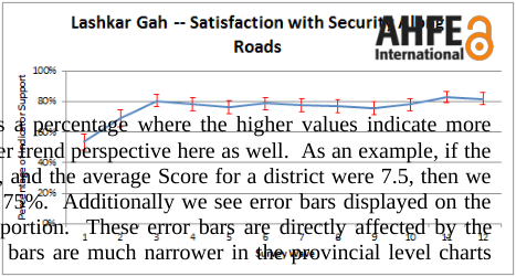
The third set of metrics displayed to the screen are charts for each district and the province showing the proportion of support for an indicator over the duration of the survey, as shown in Figures 4 and 5, regardless of the Waves selected by the user. These charts give a slightly different perspective of the indicator than shown in Figure 3. The values displayed by the line charts are again derived from the set of respondent Scores by district or province similar to Figure 3. This time, however, we are showing them as a percentage where the higher values indicate more support for the indicator; additionally we start to get a broader trend perspective here as well. As an example, if the range of unfavorable to favorable were 0 to 10, respectively, and the average Score for a district were 7.5, then we would say there proportion of support for the indicator was 75%. Additionally we see error bars displayed on the charts which represent a 95% Confidence Level of the proportion. These error bars are directly affected by the number of respondents for the survey. Therefore, the error bars are much narrower in the provincial level charts than they are in the district level charts.
Figure 4. Proportion of Support for Helmand Province Figure 5. Proportion of Support for Helmand Province As our third and final piece of the analytics suite shows in Figures 4 and 5, we can see that satisfaction with road security has been quite high in Lashkar Gah, and across Helmand Province in general, since about Wave 3 of the survey. We can now state the following from our survey data: According to Survey C the sentiment regarding the Lashkar Gah’s satisfaction with security along roads declined from Wave 4 to Wave 5, the average Lashkar Gah resident remained generally positive about road security, and that sentiment has continued to be quite steady for the duration of Survey C.
While we only have space to show a small number of indicator metrics in this paper, understand that the MICh is designed to be able to do display these metrics for all surveys in the research for any two time periods for every indicator; this equates to thousands of comparisons to be measured at the district and provincial levels of Afghanistan with only a few clicks. The metrics are relatively easy to understand and the availability of Excel to run the analytics suite is nearly universal.
CONCLUSIONS
One thing the MICh cannot do is determine the why. We can help leaders use survey data to understand popular perceptions of topics and provide them a means to use that information to formulate better decisions, but we cannot use MICh to tell us why something changed for the better or worse. To do that, one must dive even deeper into the topic of interest. In the end, the MICh serves an analytically derived exploratory data analysis tool designed to inform decisions and to incite further areas of study.
This research has demonstrated the integration of proven statistical techniques (Factor Analysis and the Mann- Whitney test) on large, complex data (surveys) into an exploratory data analysis tool that provides great potential for an organization to help understand and track a population’s perception over time. The MICh analytics suite takes the information one step further by providing quick and easy to understand metrics of the analytically derived and measured indicators. The MICh is scalable and modifiable to provide an end user a means to quickly inform leadership in a wide range of organizations when developing and analyzing long-term plans involving populations.
REFERENCES
CIA World Factbook, (2014), Afghanistan. The CIA World Factbook Website: https://www.cia.gov/library/publications/theworld-factbook/geos/af.html Conover, W. (1999). Some methods based on ranks. In W. Conover, Practical Nonparametric Statistics (pp. 269–286). New
York: John Wiley & Sons. Garrett-Mayer, E. (2006). Statistics in Psychosocial Research. Johns Hopkins University Website: Retrieved Feb 17, 2014: http://ocw.jhsph.edu/courses/statisticspsychosocialresearch/pdfs/lecture8.pdf Stuart, E. A. (2010, June). Academy Health: Advancing research, policy and practice. Retrieved Feb 19, 2014, from Academy
Health: http://www.academyhealth.org/files/2010/sunday/StuartE.pdf United States Department of Defense. (2011). Use of effects. In Commander's handbook for assessment planning and execution (p. I-8). Suffolk, VA.
Appendix
Table 7. Indicators Derived from Factor Analysis on Survey A.Table 8. Indicators Derived from Factor Analysis on Survey B.Table 9. Indicators Derived from Factor Analysis on Survey C.
LISTED IN THE AHFE DIGITAL BOOKSTORE CATALOGUE
Explore the complete digital volume
Advances in Cross-Cultural Decision Making
Read this individual research paper free through the original publisher, or explore the full digital proceedings book.
ISBN 978-1-4951-2095-4
Explore this ISBN in the AHFE Bookstore ↗Listed in the July 2026 bookstore catalogue; search by ISBN to confirm current availability · Digital book purchase optional