Vivian Egan, Elizabeth Fox (2025). A Comparison of ARIMA and XGBoost Models For Time Series Analysis Utilizing Human Behavioral Data. In: Artificial Intelligence and Social Computing. AHFE Open Access, vol. 163, pp. 204–214. https://doi.org/10.54941/ahfe1006052
Time series modeling is a powerful tool utilized across multiple domains to assess the underlying stochastic mechanisms in a dataset or to predict future values based on past values in the series. Time series forecasting has been used for many applications including the stock market, healthcare, and environmental sciences. Traditional models like ARIMA struggle with more sophisticated datasets that may have non-linear patterns, whereas more advanced machine learning models were created to handle those relationships. Despite the wide range of uses for time series modeling, use in psychology is limited. We propose by better understanding these models’ forecasting abilities with human behavioral datasets, time series can be used in various psychological and human factors applications such as monitoring and predicting behavior for improved interface design. Our work uses this tool to predict future values in a specified time trial in two human behavioral datasets. We compare the performance of ARIMA models and XGBoost models to evaluate the strengths and weaknesses of both models and establish which model performed best in our chosen evaluation metrics. Overall, ARIMA had more favorable values across performance metrics in most conditions, although XGBoost models still had well-performing scores. Although the models in our work performed well, the data needed to possess a stable mean and variance to utilize them. This requirement led to a loss of the trend throughout the time trial that was unique to each conditions’ effect on participants. Future research can utilize what we learned to work towards predictive time series models that accurately capture the unique trend of human behavioral data for more enhanced interface design
Time series analysis serves two purposes: to model the stochastic mechanism that gives rise to an observed series and to predict or forecast the future values of a series based on its history (Jebb et al., 2015). Researchers have used time series modeling across a wide variety of domains, including economics, natural sciences, and engineering (e.g., Liu, 2024a; Ariyo et al., 2014, Yadav et al., 2020; Sharma et al., 2024). Many have suggested times series modeling could also be advantageous in psychology for its predictive abilities (e.g., Jebb et al., 2015; Velicer & Fava, 2003), and offer real-time capabilities
A Comparison of ARIMA and XGBoost Models for Time Series Analysis 205
(Parpoula, 2024). However, the use of time series modeling in psychology remains limited. In the current work, we test the predictive accuracy of time series forecasting in two unique datasets with two different models.
ARIMA Models There are multiple methods for constructing time series models that vary in complexity. Autoregressive integrated moving average (ARIMA) models are the traditional choice (Hyndman & Khandakar, 2008a). ARIMA models are a type of regression analysis that operate under the assumption that a function of certain steps of past values can explain a current value in a series (Shumway et al., 2000). These models gauge the strength of one dependent variable relative to the other changing variables. ARIMA models include three parameters: autoregression (AR), integrated (I), and moving average (MA). Of particular interest in our work is the integrated term, which describes the stationarity of a dataset. Stationary data varies around a fixed mean instead of a varied one (Velicer & Fava, 2003). If the dataset is non-stationary, then it is required to difference the data to ensure it is stationary. Statistical tests such as the KPSS and the Augmented Dicky- Fuller test have been developed to evaluate if a dataset is stationary to avoid variance in the mean leading to an invalid regression (Mushtaq, 2011; Hyndman & Khandakar, 2008b). The number of rounds of differencing required is what the integrated term refers to. Human behavioral datasets often do not have fixed means. A notable downside to the ARIMA model is that these parameters are subjective. Researchers must manually define the three parameters, contributing to forecasting errors and the time investment needed to build the model (Liu, 2024).
ARIMA is a linear model, allowing it to excel only at short term and linear problems. Meaning it is usually inadequate for long-term modeling (Jebb et al., 2015). Long-term modeling is one reason ARIMA may not be the best- fit model for a dataset. ARIMA models also fall short with datasets that are composed of many interrelated variables. For example, these models excel at predicting sales and stock market analysis. These models assume linear relationships in datasets and may lead to erroneous predictions when outlier events occur, lacking flexibility for real-world applications. They also risk becoming computationally expensive with non-stationary or large datasets (Liu, 2024).
Datasets become stationary by differencing, but risk losing information. Differencing stabilizes the mean of a time series by removing change. Differenced datasets will only have T-1 values since it is impossible to calculate the difference for the first value, leading to information loss with increased differencing (Hyndman & Athanasopoulos, 2018). A complex, non-stationary dataset may include data collected using multiple measuring techniques and instruments, or a variation of short-term and long-term repeating patterns. ARIMA models may also have shortcomings in capturing complex temporal dependencies between observations, and cannot depict multiple reoccurring patterns in data (Weerakody et al., 2021).
206 Egan and Fox
Modeling Alternatives Various machine learning models have been created that use different methods to carry out time series analysis. We chose to focus on gradient boosting models due to their efficiency and success in predictive modeling in other fields (Fang et al., 2022; Zhang et al., 2021; Alim et al., 2020). Gradient boosting models allow us to randomize samples in the training and testing data set. In contrast, both neural networks and ARIMA would need the samples to be in time order and split accordingly (Chen et al., 2024). XGBoost is a gradient boosting model that outperforms similar models in Kaggle competitions (Chen et al., 2024). XGBoost’s unique feature is its ability to build an ensemble of unique models, specifically it builds many relatively weak models that work to correct the errors of previous trees to obtain a strong prediction (Natekin & Knoll, 2013). This process relies on supervised learning to find patterns in the data and generalize them to new data. The initial base models are slightly better than random guessing. Through boosting they become more accurate, reducing remaining errors to improve prediction iterations (Chen & Guestrin, 2016). In the beginning weights are spread out equally with low variance, but with each iteration, weight functions get updated where needed to reduce bias (Nielsen, 2016). This results in a model that is trained to give weight to beneficial interactions. Once trees reach max depth, they are pruned backwards until improvement in the loss function is below threshold (Sagi & Rokach, 2021). Multiple parameters are available to fine tune XGBoost’s performance and modelers may tailor them to fit their needs, making it suitable for a wide array of applications. XGBoost is also well suited to handle missing values (Chen & Guestrin, 2016). For these reasons, we chose to test this model’s accuracy to model patterns of and predict future human performance. We hypothesize that XGBoost will capture more sophisticated relationships that ARIMA models will struggle to handle. In addition, XGBoost has many customizable parameters to meet modeler needs and although it is often used with stationarity, it typically produces high predictive accuracy (Bitirgen & Filik, 2020; Lv et al., 2021). Further, we test its ability to predict two nonstationary human datasets.
METHODS
This study utilized data from two published (or under review) human experiments: 1) Adaptive Strategic Reorientation of Attention (AStRA) and Multiple Object Tracking and Communications tasks (MOTC).
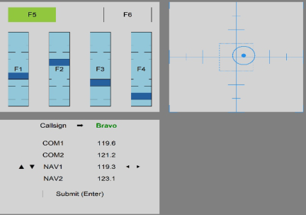
ASTRA Dataset Twenty-four participants completed different combinations of tasks from a recently developed version of the Multiple Attribute Task Battery (MATB; Fox et al), including tracking, communications, or monitoring (Figure 1). The combinations consisted of either dual task or triple tasks, with some combinations having the aid of an agent. The agent represents the cognitive countermeasure designed to reorient the participant’s attention through simple cues to enhance multitasking when deficits were detected (through
A Comparison of ARIMA and XGBoost Models for Time Series Analysis 207
brain activity). The participants completed each factorial combination for 6 minutes (Anonymous n.d.a).
Figure 1: Static image of multiple attribute task battery (MATB): monitoring (upper left), tracking (upper right), and communication (bottom left) tasks.
Multitasking throughput (MT), a measure developed by Fox et al. (2021), evaluates how well an individual performs on multiple tasks simultaneously compared to a model of their own ‘perfect timesharing’ performance. This individualized and nonparametric measure provides a single value for multitasking performance. The perfect timesharing baseline is used for comparison in computing MT; the baseline assumes task independence, meaning efficiency to complete one task is not dependent on efficiency in the other tasks, and unlimited capacity, meaning there are more resources available than demanded to complete the tasks.
For our time series prediction purposes, we wanted to estimate how MT varies over time. Fox & Houpt (2021) developed a Bayesian trial- varying model of the capacity coefficient, and we utilized the same modeling techniques as Fox & Houpt (2021) such that we assume a Weibull distribution with a fixed shape for estimating both response times and tracking error in all tasks, use a conjugate prior for computational simplicity, use a squared exponential drop-off function to compute MT over time. Like Capiola et al. (2024), Fox & Bowers (n.d.), we assume a stationary shape parameter and allow the distribution’s scale parameter to vary across individuals and time to estimate MT across trials. We calculated cost for each task in the multitask contexts, and each had a different number of events during the 6-minute time window due to the nature of the task. Generally, MT decreases as time-on-task increased; this was especially evident in tracking task performance.
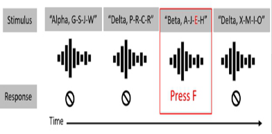
MOTC DATASET Sixteen participants completed a communication (Comms) and multiple object tracking (MOT) task with equal priority (Figure 2). The researchers manipulated the performance of the subject’s partner and how a graphical
208 Egan and Fox
interface displayed feedback information to the subject. Participants were asked to imagine they were a safety controller that relays safety information to security forces who, in turn, ensure safety at a public venue. The participants were instructed to complete the tasks remotely with eight different partners. The partners and participants were assigned to monitor one call sign for the Comms task and one quadrant for the Mot task. Scenario and tasks were adapted from previous work (Fox et al., 2024).
Figure 2: Depiction of Comms task (left) and MOT task (right).
Participants completed eight blocks of the four display types. Display types were adapted from previous work (Capiola et al., 2024). Across the eight blocks, the agent partner’s performance was manipulated with equal low and high-performance conditions. The participants could respond to their partner’s call-sign and in their partner’s quadrant. The partner could do the same for the participant.
In this study, reaction time from both tasks was used to calculate Cost for each person and task (Fox et al). When evaluating Cost across time there was not a consistent trend over time; however, the value always varied throughout the time trial.
Building the Model The authors utilized the tseries package in R (Trapletti & Hornik, 2018) to assess if the data were stationary and repeatedly differenced the data to become stationary as necessary. This was completed at the subject and condition level. Then, we fit parameters for each model. To do this we used a 70/30 split data for training/testing, respectively. For the ARIMA models, data was ordered by time. In the XGBoost Model, data was randomized.
ARIMA Model Since we differenced the data and made it stationary as our first step, we set the integrated ARIMA parameter to 0. To find the optimal choice for the remaining two parameters, we used a joint grid search ranging from zero to five (Velicer & Fava, 2003) to find the most probable p and q values. The Akaike Information Criterion (AIC) value and Root mean squared error (RMSE) assessed the performance of the models. The chosen parameters minimized these values.
A Comparison of ARIMA and XGBoost Models for Time Series Analysis 209
These performance metrics were chosen because RMSE is the recommended performance metric for XGBoost and by making this choice it allows both models to be assessed using the same metric. Additionally, AIC is a metric often used for assessing ARIMA performance, and it is used to compare the current models in a similar way to past research.
XGBoost Model XGBoost offers a wide range of customizable parameters grouped into general, booster, and learning task parameters. General parameters determine the overall function of the model. We used the default gbtree booster based on decision trees as the base learner. Booster parameters influence how the model performs each boosting iteration, allowing for fine tuning. Tree booster models have a wide variety of options, such as those we used: mtry, min n, tree depth, learn rate, loss reduction, and stop iteration. Learning task parameters allow users to define a unique loss function and establish a chosen eval metric. We did not use a unique loss function for our datasets. We selected RMSE and R2 as an evaluation metric.
To tune the parameters outlined above, we used the tidymodels package in R (Kuhn & Wickham, 2020), designed and specialized to create robust models and allowed us to tune and compare the best parameters. V-fold cross- validation, or k-fold cross-validation, is a method that randomly splits the data into V groups of similar sizes called folds. The resample of the analysis data consists of V-1 of the folds, but the assessment set contains the final fold. There are no repeats in basic V-fold cross-validation, and the number of resamples equals V (Frick et al., 2024). For our models, V was set to 5 and size set to 150. We chose these numbers because they were within the suggested range but were not too computationally expensive (Berrar, 2018).
We created and tested both ARIMA and XGBoost models and compared performance using four performance metrics. Root mean squared error (RMSE), Mean absolute percent error (MAPE), Mean absolute error (MAE), and mean absolute scaled error (MASE). R2 was calculated for XGBoost models to evaluate the fit of the model. Example plots of data are provided in the results section below.
RESULTS
Performance Metrics In the AStRA dataset, the ARIMA model outperformed the XGBoost model in almost all conditions. In some performance metrics, the XGBoost model had conditions where the performance metric was lower, meaning XGBoost was the ideal model for that condition. MAPE is the average absolute percentage difference between predicted and actual values. MAPE describes, on average, how far off the model’s predictions are from the actual values. For the MAPE performance metric, all values were greater than 50 %, which is a poor value for this metric. Values between 10 and 20 % are considered good, with models less than 10 % considered highly accurate models (Hyndman & Koehler, 2006). However, in some conditions, XGBoost had lower values.
In the MOTC dataset, the ARIMA model outperformed the XGBoost model in most conditions for all performance metrics. MAE measures the
210 Egan and Fox
average magnitude of errors between predicted and actual values without considering the direction of the errors (Hyndman & Koehler, 2006). XGBoost was lower in the one condition for the MAE performance metric, and one in the MAPE performance metric, although both models across all conditions had scores greater than 50% for this metric. MAPE values can be as low as 0%, although most are above 1%. RMSE scores were very low (indicating high predictive performance) across both models for all conditions.
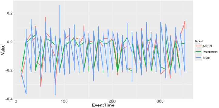
R2 relays information about the goodness of fit for the XGBoost model. In the AStRA dataset, all conditions were 0.97 or higher except for one condition, which included the tracking and monitoring tasks. R2 was both high (.80) and low to predict MOTC performance. Figure 3 shows an example of the ARIMA (top) and XGBoost (bottom) model predictions for one participant’s data in one condition of the AStRA dataset. XGBoost models provide predictions for the whole dataset, whereas ARIMA models only provide predictions for the last 30%.
Figure 3: ARIMA (top) and XGBoost (bottom) predictive model for one condition in dataset 1.
A Comparison of ARIMA and XGBoost Models for Time Series Analysis 211
DISCUSSION
In this work, we explore the performance of two time series models in predicting values in two human behavioral datasets. We sought to fill the gap in the literature pertaining to time series analysis within psychology. Throughout this study, we verified our computational methods and demonstrated that 1) time series analysis can be utilized in human behavioral data to make predictions, 2) both models in this paper can be utilized for such analysis, 3) human behavioral data must be made stationary with these models, leading to loss of trend and data. To our knowledge, this is the first study to compare similar models to those mentioned above for predictive modeling in psychology.
This study demonstrated that these models make accurate predictions, as indicated by most performance measures used. Despite ARIMA having better performance scores, XGBoost also performed at a proficient level. In future work, the XGBoost models can be refined to train a more extensive array of models across a larger grid of parameters to improve model accuracy. Furthermore, with a larger sample size XGBoost may have performed better than ARIMA. Both models had a 70/30 train/test split. However, the ARIMA model only predicted the last 30% of the data and XGBoost predicted a random 30% pulled from the full dataset. Therefore, a direct model comparison may be misleading. For instance, if time dependencies between the ARIMA datapoints are easier to predict (i.e. less variance and violate periods and more predictable patterns) its performance metrics may be artificially higher. MAPE values were poor for all models in every condition; this may be due to the values being close to zero, high variability in the data, or outliers (Hyndman & Koehler, 2006).
Previous research suggested a gap in psychological analysis methods for longitudinal data that could benefit from time series analysis, specifically predictive modeling. Previous work suggests that advances in time series could lead to near real time monitoring (Parpoula, 2024). Dynamic time series modeling in real-time would inform adaptive automation, feedback, and display optimization to enhance user performance and experience. Although currently time series analysis faces limitations in this field. Human behavioral data often is not stationary and must be made stationary to utilize these models, leading to a loss of trends that are critical to making the most accurate predictions for these complex and dynamic systems. For example, in the AStRA dataset all conditions and datasets had a downward trend not observed in the ARIMA and XGBoost models due to differencing. To remedy this and strive toward near real-time models, future work can aim to develop models that capture the trends observed in these data types (Parpoula, 2024). Work by Schumacher et al. (2023) also describes the nature of dynamic cognitive constructs such that they are affected by more than static task demands. Removing the trend from our datasets may have affected the quality of our predictions, and a model tailored to this type of data would elevate predictive performance and make models more informative for interface enhancement. Superstatistics models offer a way to manipulate both short- and long-term parameters in machine learning models to better
212 Egan and Fox
capture the nonstationary data. We suggest that future work could create a superstatistic model and utilize a gradient boosting model to improve model performance. Future work may build from our findings to push the field closer to near real-time monitoring and inform interface design based on user performance over time. This study is one of the first steps in meeting this goal.
CONCLUSION
Time series is an effective instrument for employing past data points to either understand trends among a dataset or predict future values. Time series data sets possess dependencies between observations that allow different modeling techniques to capture those relationships. This type of analysis has a broad scope of uses and disciplines. However, the use of time series analysis remains limited in psychology. We sought to fill the gap by testing ARIMA and XGBoost to predict human performance over time in two studies. Our work describes how the models vary in their customization, complexity, and test their ability to capture fluctuations in human performance over time.
Our research evaluated a traditional (ARIMA) and a machine learning (XGBoost) model to accurately predict human performance data over time. We found both models performed well above chance, but ARIMA consistently outperformed XGBoost in this use-case. Future research should investigate the use of incremental models, which may capture individual-level trends that could better adapt user’s display, provide individual- or team- level feedback, or administer enhancement techniques to elevate the user’s efficiency.
ACKNOWLEDGMENT
The views expressed are those of the authors and do not necessarily reflect the official policy or position of the Department of the Air Force, the Department of Defense, or the U.S. government. No potential conflict of interest was reported by the authors.
Distribution A. Approved for public release; distribution unlimited. AFRL- 2025-0401; Cleared 27 Jan 2025. This research was supported in part by an appointment to the Department of Defense (DOD) Research Participation Program (Vivian Egan) administered by the Oak Ridge Institute for Science and Education (ORISE) through an interagency agreement between the U.S. Department of Energy (DOE) and the DOD. ORISE is managed by ORAU under DOE contract number DE-SC0014664. All opinions expressed in this paper are the author’s and do not necessarily reflect the policies and views of DOD, DOE, or ORAU/ORISE.
REFERENCES
Alim, M., Ye, G.-H., Guan, P., Huang, D.-S., Zhou, B.-S. & Wu, W. (2020), ‘Comparison of arima model and xgboost model for prediction of human brucellosis in mainland China: A time-series study’, BMJ open 10(12), e039676.
A Comparison of ARIMA and XGBoost Models for Time Series Analysis 213
Fox, E.L., Stephenson, A., Vivian, E., Bowers, G., & Ugolini, M.(n.d.a), Adaptive strategic reorientation of attention. In preparation. Fox, E., Capiola, A., Stephenson, A., Bowers, G., Harris, K.,& Egan, V., (n.d.b), The
effects of teammate performance and display type on real-time team multitasking throughput. Submitted to journal for review. Ariyo, A. A., Adewumi, A. O. & Ayo, C. K. (2014), Stock price prediction using the arima model, in ‘2014 UKSim-AMSS 16th international conference on computer modelling and simulation’, IEEE, pp. 106–112. Berrar, D. (2018) ‘Cross-Validation,’ in Elsevier eBooks, pp. 542–545. https://doi.org/
10.1016/b978-0-12-809633-8.20349-x. Bitirgen, K. & Filik, U. B. (2020), ‘Electricity price forecasting based on xg-¨boost and arima algorithms’, BSEU Journal of Engineering Research and Technology 1(1), 7–13. Capiola, A., Fox, E. L., Bowers, G., Harris, K. N. & Woods, S. (2024), Investigating
interfaces that convey team efficiency, in ‘2024 IEEE 4th International Conference on Human-Machine Systems (ICHMS)’, IEEE, pp. 1–6. Chen, T. & Guestrin, C. (2016), Xgboost: A scalable tree boosting system, in ‘Proceedings of the 22nd acm sigkdd international conference on knowledge discovery and data mining’, pp. 785–794. Chen, T., He, T., Benesty, M., Khotilovich, V., Tang, Y., Cho, H., Chen, K., Mitchell,
R., Cano, I., Zhou, T., Li, M., Xie, J., Lin, M., Geng, Y., Li, Y. & Yuan, J. (2024), xgboost: Extreme Gradient Boosting. R package version 1.7.8.1. URL: https:// CRAN. R-project.org/package=xgboost Fang, Z.-g., Yang, S.-q., Lv, C.-x., An, S.-y. & Wu, W. (2022), ‘Application of a datadriven xgboost model for the prediction of covid-19 in the USA: A time-series study’, BMJ open 12(7), e056685. Fox, E. L., Capiola, A., Bowers, G. and Stephenson, A. (2024). A metric of team
multitasking throughput. Journal of Experimental Psychology: Applied, 31(1), pp. 58–70. doi: https://doi.org/10.1037/xap0000519 Fox, E. L. & Bowers, G. (n.d.), Real-time prediction of attention and performance using neural activity. Fox, E. L. & Houpt, J. W. (2021), ‘A bayesian model of capacity across trials’, Journal
of Mathematical Psychology 105, 102604. Fox, E. L., Houpt, J. W. & Tsang, P. S. (2021), ‘Derivation and demonstration of a new metric for multitasking performance’, Human Factors 63(5), 833–853. Frick, H., Chow, F., Kuhn, M., Mahoney, M., Silge, J. & Wickham, H. (2024),
rsample: General Resampling Infrastructure. R package version 1.2.1, https:// github.com/tidymodels/rsample. URL: https://rsample.tidymodels.org Hyndman, R. & Athanasopoulos, G. (2018), Forecasting: Principles and Practice, 2nd edn, OTexts, Australia. Hyndman, R. J. & Khandakar, Y. (2008a), ‘Automatic time series forecasting: the
forecast package for R’, Journal of Statistical Software 27(3), 1–22. Hyndman, R. J. & Khandakar, Y. (2008b), ‘Automatic time series forecasting: The forecast package for r’, Journal of Statistical Software 27(3), 1–22. URL: https:// www.jstatsoft.org/index.php/jss/article/view/v027i03. Hyndman, R. & Koehler, A. (2006), ‘Another look at measures of forecast accuracy’,
International Journal of Forecasting 22, 679–688. Jebb, A. T., Tay, L., Wang, W. & Huang, Q. (2015), ‘Time series analysis for psychological research: Examining and forecasting change’, Frontiers in psychology 6, 144575.
214 Egan and Fox
Kuhn, M. & Wickham, H. (2020), Tidymodels: A collection of packages for modeling and machine learning using tidyverse principles. URL: https:// www.tidymodels.org. Liu, J. (2024a), ‘Navigating the financial landscape: The power and limitations of the arima model’, Highlights in Science, Engineering and Technology 88, 747–752. Liu, J. (2024b), ‘Navigating the financial landscape: The power and limitations
of the arima model’, Highlights in Science, Engineering and Technology 88, 747–752. URL: https://drpress.org/ojs/index.php/HSET/article/view/19082. Lv, C.-X., An, S.-Y., Qiao, B.-J. & Wu, W. (2021), ‘Time series analysis of hemorrhagic fever with renal syndrome in mainland China by using an XGBoost forecasting model’, BMC infectious diseases 21, 1–13. Mushtaq, R. (2011) ‘Augmented Dickey Fuller test,’ SSRN Electronic Journal. https://
doi.org/10.2139/ssrn.1911068. Natekin, A. & Knoll, A. (2013), ‘Gradient boosting machines, a tutorial’, Frontiers in neurorobotics 7, 21. Nielsen, D. (2016), Tree boosting with XGBoost-why does XGBoost win” every”
machine learning competition?, Master’s thesis, NTNU. Parpoula, C. (2024), ‘An analytical approach for identifying trend-seasonal components and detecting unexpected behaviour in psychological time-series’, International Journal of Psychology 59(6), 1307–1316. Sagi, O. & Rokach, L. (2021), ‘Approximating XGBoost with an interpretable decision tree’, Information sciences 572, 522–542. Sharma, A. K., Punj, P., Kumar, N., Das, A. K. & Kumar, A. (2024), ‘Lifetime
prediction of a hydraulic pump using arima model’, Arabian Journal for Science and Engineering 49(2), 1713–1725. Shumway, R. H., Stoffer, D. S. & Stoffer, D. S. (2000), Time series analysis and its applications, Vol. 3, Springer. Trapletti, A. & Hornik, K. (2018), tseries: Time Series Analysis and Computational
Finance. R package version 0.10–43. URL: https://CRAN. R-project.org/ package=tseries. Velicer, W. F. & Fava, J. L. (2003),’Time series analysis’, Research methods in psychology 2. Weerakody, P. B., Wong, K. W., Wang, G. & Ela, W. (2021), ‘A review of irregular
time series data handling with gated recurrent neural networks’, Neurocomputing 441, 161–178. Yadav, A. K., Das, K. K., Das, P., Raman, R. K., Kumar, J. & Das, B. K. (2020), ‘Growth trends and forecasting of fish production in assam, india using arima model’, Journal of Applied and Natural Science 12(3), 415–421. Zhang, L., Bian, W., Qu, W., Tuo, L. & Wang, Y. (2021), Time series forecast of sales
volume based on XGBoost, in ‘Journal of Physics: Conference Series’, Vol. 1873, IOP Publishing, p. 012067.
LISTED IN THE AHFE DIGITAL BOOKSTORE CATALOGUE
Explore the complete digital volume
Artificial Intelligence and Social Computing
Read this individual research paper free through the original publisher, or explore the full digital proceedings book.
ISBN 978-1-964867-39-7
Explore this ISBN in the AHFE Bookstore ↗Listed in the July 2026 bookstore catalogue; search by ISBN to confirm current availability · Digital book purchase optional