Keiichi Watanuki, Tetsuhiro Suzuki, Yusuke Osawa, Kazunori Kaede, Shinsuke Kazama (2022). Automatic Generation of AI-based Cancer Pathology Data and Highly Accurate Colorectal Cancer Pathology Diagnosis Support. In: Affective and Pleasurable Design. AHFE Open Access, vol. 41, pp. 111–119. https://doi.org/10.54941/ahfe1001787
Owing to the increase in the number of pathological diagnoses and the shortage of pathologists, the burden on pathologists has been increasing. Accordingly, support systems are expected to be utilized for analyzing pathological images using deep learning to reduce the burden on pathologists. However, the deep learning model needs to be trained using a dataset consisting of a large number of cases, to improve its performance. However, the creation of such a dataset is labor-intensive and time-consuming. Thus, an efficient method for creating datasets is required to create large datasets for future practical use. In this paper, we propose a method for creating datasets using image segmentation based on deep learning. First, we investigated whether the discriminative performance of the deep learning model can be improved by using a narrow-band light source for photographing pathological specimens. Consequently, the correct response rate was 0.93 when a white LED was used as the light source and the image was used as the input, and 0.95 when two narrow-band light sources of wavelengths 500 nm and 570 nm were used as the light sources and the image was used as the input. This indicates that using a specific narrow-band light source can improve the discrimination performance of the deep learning model compared with using white LEDs as the light source. In addition, we efficiently constructed a large and precise dataset consisting of 1018 colorectal pathology images (2028 images) and pixel-by-pixel annotation information using a dataset creation method based on image segmentation via deep learning. In contrast to the conventional handwritten annotation process, which takes an average of 520 s, the proposed method takes an average of 137 s; thus, the creation of the database is accelerated. We trained a deep learning model using the dataset of colorectal pathology specimen images created in this study. The deep learning model was trained to classify images obtained by segmenting the large-sized pathological specimen images into those containing malignant tumors and those not containing malignant tumors. The results of the diagnostic accuracy of the model were as follows: a sensitivity of 95.2%, a specificity of 97.1%, a positive predictive value of 95.29%, and a negative predictive value of 97.06%. The percentage of correct classification was 0.97, and the AUC was 0.99. In this study, we constructed a pathological specimen imaging system using narrow-band light sources of two specific wavelengths as the imaging light source, and created a dataset with high accuracy semi-automatically via image segmentation using deep learning. In addition, we constructed a system that can efficiently and semi-automatically create a large and precise dataset consisting of colorectal pathology images and pixel-by-pixel annotation information. We evaluated these systems and confirmed that they could classify colorectal pathology specimen images as accurately and quickly as or more accurately than pathologists. Thus, we demonstrated their usefulness as a pathology image analysis support system.
In recent years, the number of cancer cases and deaths due to cancer has been increasing worldwide. According to global cancer statistics (Sung et al. 2020), colorectal cancer is one of the leading causes of cancer and mor- tality, ranking fourth for the total number of cancer cases and second for the total number of deaths in men and women. The number of new cases of colorectal cancer in 2018 was 1148515 and the number of deaths was 576858. Histopathological diagnosis was performed by a pathologist who obse- rved the tissue and cells of the lesion obtained from the patient’s body under a microscope. Currently, the number of pathologists is overwhelmingly small compared with the increasing number of histopathological diagnoses, where the burden on pathologists is becoming a serious problem. To solve this problem, a histological image analysis system using a convolutional neu- ral network (CNN) (Lecun, 1998) is effective. Research on the histological image analysis using CNNs has been actively conducted, including tumor classification, segmentation, and outcome prediction. Spanhol et al. created a CNN odel to classify benign and malignant tumors of breast cancer using the BreakHis dataset (Spanhol et al. 2015), which consists of histological images of 82 breast cancer patients; and achieved an accuracy of appro- ximately 90.0% (Spanhol et al. 2016). Raczkowski et al. created a deep learning model to classify benign and malignant tumors using 10 histopa- thological tissue slides of colorectal cancer from anonymous patients, and achieved 99.1% accuracy (Raczkowski et al. 2019). They also developed a CNN model that classified eight classes: tumor epithelium, simple stroma, complex stroma, immune cells, debris (including necrosis, hemorrhage, and mucus), normal mucosal glands, adipose tissue, and background, achieving a 92.4% accuracy. Stoean et al. used a dataset of 357 histopathological slides of colorectal cancer to classify cancer grades using a CNN model that automa- tically tunes hyper-parameters, achieving an accuracy of 92.0% (Stoean et al. 2020). To improve the generalization performance of the CNN model, it was necessary to train the model using a wide variety of samples. However, in most of the previous studies, the models were trained using datasets with a relatively small number of cases. One of the reasons for the small number of cases in the dataset is that it is time consuming to create a dataset consisting of many cases. Iizuka et al. created two datasets consisting of 4628 WSIs for gastric tumors and 4536 WSIs for colorectal epithelial tumors, all of which were manually annotated by pathologists (Iizuka et al. 2020). However, to create large datasets for future practical use, it is necessary to develop an efficient method for dataset creation. In this study, we proposed a method for dataset creation using deep learning-based image segmentation and con- structed a large and precise dataset consisting of 1018 colorectal histology images (2028 images) and pixel-by-pixel annotation information using the proposed method. We also investigated the effect of narrow-band light as a light source for histopathological imaging on the recognition performance of the CNN model.
Automatic Generation of AI-Based Cancer Pathology Data 113
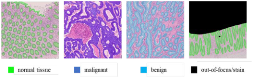
Figure 1: Example of an image with four types of annotation information assigned to each pixel: normal tissue, malignant tumor, benign tumor, and out-of-focus/stain.
CREATING A DATASET OF COLORECTAL HISTOLOGY IMAGES To construct a histopathological diagnosis model using deep learning, we need a dataset of histological images with detailed annotations consisting of various samples. However, such a dataset is time-consuming. Therefore, we have developed an efficient dataset construction method based on image segmentation. In this study, we used 2028 colorectal histology images of 1018 cases provided by the Saitama Cancer Center. Each pixel in the histology ima- ges was assigned one of four types of information: malignant tumor, benign tumor, normal tissue, other, and out-of-focus/stain, as shown in Figure. 1. The flow of the annotation process using image segmentation is as follows: First, the histological image is divided into foreground and background regi- ons by image segmentation. The foreground region is one of the regions of malignant tumors, benign tumors, and normal tissue; and the background region comprises the rest of the regions. The operator, under the guidance of a physician, assigns an appropriate pathological category to the foreground region obtained by image segmentation. The operator also hand-corrects the image if necessary. The average time required for the annotation process was 520 s when one operator performed conventional handwriting annotations in six cases, where the average time required for the annotation process using image segmentation in 103 cases was 137 s. As a result, the time required for annotation using image segmentation was reduced compared with that required for handwriting.
TRAINING AND EVALUATION OF A COLORECTAL CANCER RECOGNITION MODEL A colorectal cancer recognition model was constructed using a dataset cre- ated based on 2028 images of colorectal histopathological slides from 1018 cases. When the annotation was completed for all 2028 pathological ima- ges, the ratio of the area occupied by the pixels of each category to the entire dataset is shown in Table 1, and the number of images containing the pixels of each class is shown in Table 2. In this study, we trained a two- class recognition model with malignant tumor regions as “cancer-containing” images and the other regions as “cancer-free” images; and evaluated its performance.
The trained model was evaluated using a test dataset, and the correct response rate, which is a measure of the percentage of correct predictions
Table 1. Percentage of area occupied by each category relative to the entire data set [%].
Table available in the original PDF paper.
Malignant Benign Normal tissue Other Out-of-focus/stain
19.7 0.860 14.1 60.6 4.76
Table 2. Number of images in each category.
Table available in the original PDF paper.
Malignant Benign Normal tissue Other Out-of-focus/stain
905 91 1027 2028 430
Table 3. Confusion matrix of the colorectal cancer recognition model.
Table available in the original PDF paper.
Prediction Positive Negative
Truth Positive 1907 106 Negative 52 2646
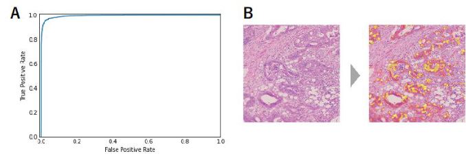
among all the predictions, was 0.9665. The sensitivity, which is a measure of the proportion of all images containing cancer that the model correctly predi- cted as containing cancer, was 0.947. Specificity, a measure of the proportion of all cancer-free images that the model correctly predicted as cancer-free, was 0.981. The goodness of fit, which is a measure of the proportion of ima- ges that the model correctly predicted as containing cancer, was 0.973. The discrimination threshold for calculating these values was set to 0.5. Table 3 summarizes the inference results of the trained model on the test dataset and their correctness as a confusion matrix. The receiver operating characteri- stic (ROC) obtained by plotting the false positive rate and the true positive rate for different discrimination thresholds is shown in Figure 2A. The area under the ROC curve (AUC was the best when the value was 1) was 0.994, indicating the recognition performance of the model.
For the trained model, we performed feature visualization using Grad- CAM, which is an algorithm for visualizing the part of an image input for a CNN model that contributes to the inference results, and can visualize the feature area for each category as a heat map (Selvaraju et al. 2017). In this study, we used Grad-CAM to visualize and identify regions where cancer features exist in the histological images. Even when the output score of the model (the value that indicates the presence of cancer in the image) is low, the visualization results using Grad-CAM can prompt the pathologist to confirm the presence of cancer and prevent oversight.
Figure 2B shows an example of an application of Grad-CAM to the infe- rence of a trained model on a histological test image. The yellow areas on the heatmap indicate the influence of the model on the output (probability that the image contains cancer).
Automatic Generation of AI-Based Cancer Pathology Data 115
Figure 2: (A) ROC curve of the colorectal cancer recognition model trained on a data- set of 2028 colorectal histology images from 1018 cases and evaluated on the test data. (B) Example of the visualization of cancer features using Grad-CAM in the trained model.Table 4. Confusion matrix of the model using different narrow-band lights.
TRAINING AND VALIDATION OF A DEEP LEARNING MODEL USING TWO TYPES OF IMAGES CAPTURED USING DIFFERENT NARROW-BAND LIGHTS AS INPUT A deep learning model was constructed using images taken using two diffe- rent narrow-band light sources as inputs for 325 combinations of 26 different narrow-band lights, selecting two without overlap. The output of the model was a two-class recognition of “with cancer” or “without cancer”. Using this model, we compared the recognition performance of two different combina- tions of input images with two narrow-band light sources. The performance of the model was evaluated using five-part cross-validation.
The highest average rate of 0.948 was obtained for the combination of narrow-band light sources with a peak wavelength of 500 nm and narrow- band light with a peak wavelength of 570 nm. The sensitivities and spe- cificities of the models trained using images taken with narrow-band light sources peaking at 500 and 570 nm, and the model trained using two types of images taken with narrow-band light sources peaking at these two different wavelengths, are shown in Table 4.
DISCUSSION
In the present annotation, the same category of information was assigned to all pixels in a single malignant tumor region. However, it is considered that there are some areas in the malignant tumor that show the characteri- stics of cancer, such as nuclear atypia and structural atypia, and some areas that do not. Therefore, it is possible that when the image is segmented, only
Table 5. Confusion matrix.
Table available in the original PDF paper.
Prediction Positive Negative
Truth Positive 91 0 Negative 7 99
areas that do not contain many cancer features are included in the image. In this case, the correct label is “contains cancer” even though the segmen- ted image does not contain many features of cancer. It is considered that the CNN model predicts “does not contain cancer” for such images, resulting in false negatives. In addition, in this label assignment method, if the segmented image contains a malignant tumor, the label of the segmented image will be “contains cancer” only. However, it is possible that not only the malignant tumor itself, but also the surrounding tissues and tissues that do not directly contain the malignant tumor, are affected by the malignant tumor and may be learned by the deep learning model as features of cancer. Therefore, it is considered that false positives are generated by predicting “contains cancer” for images that do not contain malignant tumors but contain tissues affected by malignant tumors (the correct answer label is “does not contain cancer”). We calculated the main prediction label of one image before segmentation and compared it with the main label of one image before segmentation; where the confusion matrix is shown in Table 5.The main predictive label of one image before segmentation was “contains cancer” if any of the predi- ctive labels of the trained deep learning model for each of the 25 segmented images contained “contains cancer,” and “does not contain cancer” if oth- erwise. The main label of one image before segmentation was “contains cancer” if the image contained a malignant tumor region, and “does not con- tain cancer” if otherwise. Table 5 shows that the sensitivity of the diagnosis using this deep learning model is 100%, suggesting that a histopathologi- cal diagnosis system using deep learning may be able to make a diagnosis of histological images with high accuracy without overlooking malignant tumors.
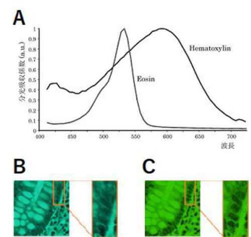
Next, we consider the recognition performance of the deep learning model in relation to the light source when photographing the histopathological sli- des. In HE staining, the cytoplasm is stained pink with eosin dye (hereinafter referred to as “E dye”) and the nuclei are stained blue with hematoxylin dye (hereinafter referred to as “H dye”) (Yamaguchi, 2015). Figure 3A shows the spectral absorption coefficients of the E and H dyes. Figure 3A shows absorption peaks near 530 and 590 nm for the E and H dyes, respectively. In the training of the deep learning model with a single input of histology images taken using narrow-band light as the light source, a high average correct response rate was obtained when the peak wavelength of the narrow- band light was between 480 and 560 nm. Since both the E-dye and H-dye are absorbed well at wavelengths in this range, the nuclei and cytoplasm of cells appeared darker in the histological images taken with narrow-band light peaking at these wavelengths; and both nuclear and structural atypia,
Automatic Generation of AI-Based Cancer Pathology Data 117
Figure 3: (A) Spectral absorption coefficients of H- and E-dyes (Yamaguchi, 2015) (B) Example images of a histopathological slide taken using a wavelength of 500 nm as a light source (C) Example images of a histopathological slide taken using a wavelength of 570 nm as a light source.
which are characteristic of colorectal cancer, can be observed more clearly. Therefore, a deep learning model with higher recognition accuracy than other methods may have been obtained.
In the training of the deep learning model using two types of images taken with different narrow-band light sources as input, we obtained a higher ave- rage rate of correctness for 17 combinations of narrow-band light sources than those of the deep learning model using images taken with white light sources as input. All 17 combinations use narrow-band lights with peak wavelengths of 500 nm or 510 nm, and narrow-band lights with peak wave- lengths of 400–420 nm or 550–650 nm. The wavelengths of 500 nm and 510 nm have relatively high absorption coefficients for both the E and H dyes, while the wavelengths of 400–420 nm and 550–650 nm have relatively low absorption coefficients for the E-dye. Yuzuki et al. reported that the dif- ference in stainability of HE staining was mostly due to the staining attitude of the E-dye (Yugi et al. 2016). Therefore, by combining images taken using the band with a low absorbance of E-dye with images taken using the band with a high absorbance of E- and H-dyes and using them for learning, the model becomes more resistant to variations in staining.
In addition, if we look at the sensitivity and specificity in Table 4, 500 nm is included in the band between 480 nm and 560 nm, where the ave- rage correctness rate was high in the model with one condition of image as input, suggesting that the CNN can discriminate cancer cells based on nuclear and structural atypia, which are characteristics of colorectal cancer,
and thus has high sensitivity. Additionally, by also using wavelengths in the band where both the E-dye and H-dye absorb light well, the sensitivity can be similarly increased. However, at 500 nm, many images containing gland ducts, as shown in Figure 3B, were misrecognized as images containing cancer cells. In contrast, at 570 nm, these images were correctly recognized, and the specificity was high. This may be due to the fact that the shape of each cell nucleus became clear at 570 nm, as shown in Figure. 3C, and because the light absorption in the cytoplasm was low, it was possible to recognize that the nuclei were normal. In addition, we believe that the specificity can be increased not only at 570 nm, but also by using wavelengths in the band where the H dye absorbs lighter than the E dye.
Therefore, by combining two types of images taken with light in the bands where both the E-dye and H-dye absorb light well (500 nm and 510 nm) and in the bands where the H-dye absorbs light lighter than the E-dye (400–420 nm and 550–650 nm), it is possible to obtain images with high sensitivity and specificity that are resistant to staining variation. This deep learning model has higher sensitivity and specificity, and is more robust to staining variation than the deep learning model trained using images taken with white light or one type of narrow-band light source.
CONCLUSION
In this study, we constructed a pathological specimen imaging system using narrow-band light sources using two specific wavelengths as the imaging light source, and semi-automatically created a dataset with high accuracy via image segmentation using deep learning. In addition, we constructed a system that can efficiently and semi-automatically create a large and precise dataset comprising colorectal pathology images and pixel-by-pixel annota- tion information. We evaluated these systems and confirmed that they could classify colorectal pathology specimen images as accurately and quickly as, or more accurately than, pathologists. Thus, we demonstrated their usefulness as a support system for pathological image analysis.
REFERENCES
Iizuka, O., et al., “Deep Learning Models for Histopathological Recognition of Gastric and colonic epithelial tumours”, Scientific Reports, Vol. 10, No. 1 (2020), pp. 1–11. Lecun, Y., “Gradient-based learning applied to document recognition”, Proceedings
of the IEEE, Vol. 86, Issue 11(1998), pp. 2278–2324. Rçczkowski, Ł., et al., “ARA: accurate, reliable and active histology image recognition framework with Bayesian deep learning”,Scientific reports, Vol.9, No. 1 (2019), pp. 1–12. Ronneberger, O., Fischer, P., and Brox, T., “U-net: Convolutional networks
for biomedical image segmentation”, In International Conference on Medical image computing and computer-assisted intervention, Springer, Cham, (2015), pp. 234–241. Selvaraju, R. R., et al., “Grad-cam: Visual explanations from deep networks via gradient-based localization”, The IEEE International Conference on Computer Vision (ICCV), (2017), pp. 618–626.
Automatic Generation of AI-Based Cancer Pathology Data 119
Spanhol, F. A., Oliveira, L. S., Petitjean, C., and Heutte, L., “A dataset for breast cancer histology image recognition”, IEEE Transactions on Biomedical Engineering, Vol.63 No. 7 (2015), pp. 1455–1462. Spanhol, F. A., Oliveira, L. S., Petitjean, C., and Heutte, L., “Breast cancer histology
image recognition using Convolutional Neural Networks”, 2016 international joint conference on neural networks (IJCNN). IEEE, (2016), pp. 2560–2567. Stoean, R., “Analysis on the potential of an EA–surrogate modelling tandem for deep learning parametrization: an example for cancer recognition from medical ima- ges”, Neural Computing and Applications,Vol. 32, No. 2 (2020), pp. 313–322. Sung, H., Ferlay, J., Siegel, R. L., Laversanne, M., Soerjomataram, I., Jemal, A., &
Bray, F.,”Global cancer statistics 2020: GLOBOCAN estimates of incidence and mortality worldwide for 36 cancers in 185 countries”,CA: a cancer journal for clinicians,Vol. 71, No. 3 (2021), pp. 209–249. Yamaguchi, Y., “Multispectral Image Analysis for Pathology”, The journal of the institute of image information and television engineers, Vol. 69, No. 5 (2015), pp. 432–436. Yugi, H., et al., “Fundamental study on control of stainability of hematoxylin-eosin
staining using a spectrophotometer”, Japanese journal of medical technology, Vol. 65, No. 3 (2016), pp. 251–259.
LISTED IN THE AHFE DIGITAL BOOKSTORE CATALOGUE
Explore the complete digital volume
Affective and Pleasurable Design
Read this individual research paper free through the original publisher, or explore the full digital proceedings book.
ISBN 978-1-958651-17-9
Explore this ISBN in the AHFE Bookstore ↗Listed in the July 2026 bookstore catalogue; search by ISBN to confirm current availability · Digital book purchase optional