Norbert L. Brodtmann, Daniel Schilberg (2023). Kinematics of Serial Robotics - Algorithms for simplified calculation of Direct & Inverse Kinematics in a Consistent Coordinate Reference system. In: Emerging Technologies and Future of Work. AHFE Open Access, vol. 117, pp. 163–177. https://doi.org/10.54941/ahfe1004416
A novel algorithm structure of direct and inverse kinematics for the motion calculation of articulated robots is presented. These algorithms are based on a 3D rotation matrix, which is known in itself but not established in robotics, as well as the principle of a normalized vector orientation, introduced here. The algorithms can handle any number of rotation and telescop axes, can be fully parameterized according to individual hardware and are also much clearer than the established & classic Denavit-Hartenberg conventions.State of the art According to current research (2022/23), the (published) robot mathematics are still based on the classical Denavit-Hartenberg conventions from 1955, which formalize the calculation of the "Direct" kinematics. For this purpose, they require a separate Local Coordinate System (LCS) for each robot arm in addition to the stationary (world) reference coordinate system. On the one hand, the spatial position of individual links to each other is therefore not directly comparable. On the other hand, the movement of a single robot arm changes the spatial point position of each following link in the kinematic chain accordingly - which is not represented by the LCS.For decades, the DH conventions have been considered state of the art for forward and direct kinematics in science and technology. Standard algorithms for backward and inverse kinematics, however, have not been disclosed to the general public. Companies that manufacture robots consider the computational core of their own algorithms to be a "trade secret". Only the operator level is published.Solution approachIn this paper, a general inverse kinematics trajectory control algorithm for serial robot systems (articulated arm and SCARA) is presented. These algorithms systematically avoid the problem of uncontrolled singularity of inverse kinematics. The combination of similar rotation matrices working consistently in the (world) reference coordinate system as well as the normalized vector orientation – introduced in this work – offer a number of advantages. They not only allow a doubtless parameter assignment without danger of confusion of the two length parameters required for each DH matrices. It becomes possible to specify a generally valid algorithm of inverse kinematics for trajectory control.The solution to be published here does not require any additional location coordinates for each moving robot element, it consistently references one and the same (world) reference coordinate system. Any vector position and its orientation in 3D-Space can be compared directly - an essential prerequisite for the snapping algorithms of the inverse kinematics also disclosed here and the additional option of an integrated traversability of the robot on the gantry system. The consistency of the coordinate system enables perspective representation in imaging processes.The vector input values required for this are directly available – in the (world) reference coordinate system (CRS) – for each point of the kinematic chain.For hardware control, kinematic angular values of the robot arm movement are output via a motion protocol. A specially developed simulation visualizes the moving robot silhouette and the path to be traced in a freely selectable perspective.
In this paper, a general inverse kinematics trajectory control algorithm for serial robot systems (articulated arm and SCARA) is presented. These algorithms systematically avoid the problem of uncontrolled singularity of inverse kinematics. The combination of similar rotation matrices work- ing consistently in the (world) Coordinate Reference System (CRS) as well as the Normalized Vector Orientation – introduced in this work – offer a number of advantages. They not only allow a doubtless parame- ter assignment without danger of confusion of the two length parameters required for each DH matrices. It becomes possible to specify a gener- ally valid algorithm of inverse kinematics for continuous path control. Last but not least the algorithm offers the possibility to calculate ball joints.
The solution to be published here does not require any additional location coordinates for each moving robot element, it consistently references one and the same (world) Coordinate Reference System (CRS). Any vector position and its orientation in 3D-space can be compared directly - an essential pre- requisite for the snapping algorithms of the inverse kinematics also disclosed here and the additional option of an integrated traversability of the robot on the gantry system. The consistency of the coordinate system enables perspec- tive rendering in imaging processes. The vector input values required for this are directly available – in the Coordinate Reference System (CRS) – for each point of the kinematic chain.
For hardware control, kinematic angular values of the robot arm move- ment are output via a motion protocol. A specially developed simulation visualizes the moving robot silhouette and the path to be traced in a freely selectable perspective.
State of the Art According to current research (2022/23), the (published) robot mathemat- ics are still based on the classical Denavit-Hartenberg conventions from 1955, which formalize the calculation of the “Direct” kinematics. For this purpose, they require a separate Local Coordinate System (LCS) for each robot arm in addition to the stationary Coordinate Reference System (CRS). (Kreuzer, 1994) as well as (Weber, 2013) explain the assignment of Cartesian Coordinate systems to the robot mechanics by means of the DH matrix [1_01], using an individual Local Coordinate System (LCS) for each link.
A well-known handicap is, on the one hand, that the LCS does not allow a direct comparison of the spatial position of individual links among each other. On the other hand, the movement of a single robot arm changes the spatial point position of each following link in the kinematic chain accordingly - which is not represented by the LCS. For decades, the DH conventions have been considered state of the art for forward and direct kinematics in science and technology. Standard algorithms for backward and inverse kinematics, however, have not been disclosed to the general public. Companies that man- ufacture robots consider the computational core of their own algorithms to be a “trade secret”.
Due to limited space of this paper, just a few milestones of DH con- ventions and its matrix can be pointed out here. In the Springer Hand- book of Robotics, (2016) Prof. Kenneth J Waldron, and Prof. James Schmiedeler describe under 2.4 Geometric Representation not only the basic convention according to Denavit Hartenberg to transfer a LCS of the kinematic chain into a neighboring one. The authors also deal inten- sively with the difficulties of the DH parameter assignment, which led to adaptations and modification according to Khalil and Dombre (2.44) / Waldron and Paul as well as Craig. Since DH modification is not the focus of this paper, the classical well known DH matrix is shown under [1_01].
Kinematics of Serial Robotics Algorithms for Simplified Calculation 165
The DH matrix - whether original, cf. [1_01] or modified – is a 4x4 matrix with homogeneous coordinates referenced to xyz in column 4. It uses 2 different length parameter (mostly called “a” and “d”) and two angles (“α” and “θ”). “α” indicates the orientation of the rotation axis, “θ” is the operative angle of the rotation. The orientation can be in alignment (α = 0) or perpendicular to the support arm (+/−π/2). The formula val- ues “a” and “d” are measures of length. Whether the length of an arm link is to be assigned to the parameter “a” or “d” is one of the tech- nical difficulties of the DH system - with enormous impact on “xyz” in the LCS.
The DH system describes the vector orientation of a robot arm link not directly as a vector orientation in 3D space but relatively as an angle between two successive LCS links. To transfer the LCS chain into the Coordinate Ref- erence System (CRS) - which defines the position of the workpiece to be processed - the individual DH matrices are multiplied together. To become familiar with the Denavit-Hartenberg system needs a lot of experience and skill.
Aim of This Elaboration is not to show simpler rules of the DH-parameter assignment. The aim is to present a calculation system of the kinematics that does not require these complicated assignments, especially since it offers very simple solutions of Inverse Kinematics as it uses entirely the (world) Coordinate Refer- ence System (CRS), - here better called Consistent Coordinate Reference system (CCR).
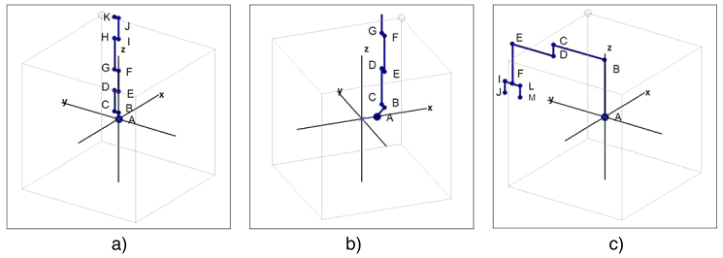
True 3D-Transformation The method presented here works with real 3D rotation matrices. At first sight, the operational calculation effort is higher than with DH, but the 3D matrices are very flexible and can be handled without any risk of con- fusion due to wrong parameter assignment. In spirit of universality, the algorithms described here do not distinguish between robot arms (swivel axes) and their rotational axes. The Normalized Vector Orientation (pl. see Fig. 2/3) introduced in connection with the R3 Rotation Matrix [2_02] make it possible to define all parts consistently as axis and to assign to them arbitrary swivel or rotation function or both. The axes are labeled - independent of their function - according to their position in the kine- matic sequence with the start- and target-points of their vectors, cf. spa- tial point definition of the kink points A/B/C/D/E in 3 dimensional space (Fig. 1).
166 Brodtmann and Schilberg
Figure 1: Robot silhouette in “home position”, modeled by Normalized Vector Orienta- tion. Fig. 1 a) Axis A/B foot point angle 0◦. Fig. 1 b) Axis A/B 45◦, in addition: optional x offset of footpoint A. Fig. 1 c) SCARA with optional end effector Please note: Rotation of axis A/B is independent of the footpoint angle always by “z”. If axis A/B: has an offset (Fig. 1 b), rotation is parallel to “z”.
By definition (pl. see Fig. 1),
every transition point from one vector to the next is marked alpha- betically from the letter sequence ABC - starting with “A” at the fix point
a vector end point of a link is at the same time the start point of the cascading following one,
each chain link, regardless of whether it is a rigid arm or an articulated axis, is labeled with a double letter (e.g., C/D). A shared point (for exam- ple, “D”) therefore connects neighboring links (for example, C/D with D/E).
Consistent Coordinate Reference System & Normalized Vector Orientation The system does not require additional Location Coordinates systems (LCS) for each moving robot limb, the R3-Rotation Matrices consistently refer to one and the same Consistent Coordinate Reference system (CCR). The zero point definition does not refer to a theoretical matrix zero points, but to the real mechanical zero points of the arm joints.
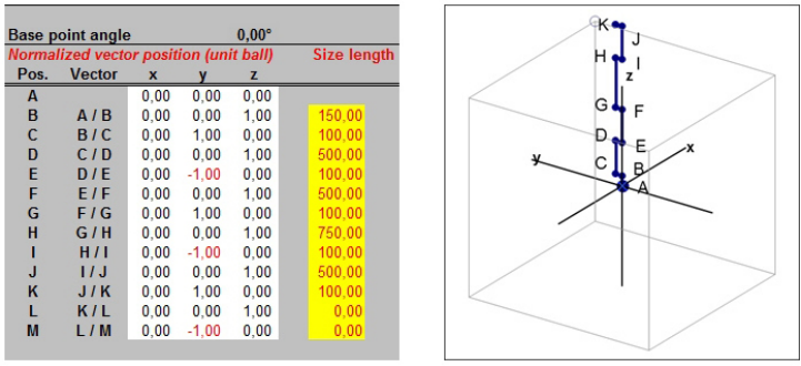
Per unit sphere, the Normalized Vector Orientation describes the orienta- tion of each kinematic chain link in the Consistent Coordinate Reference sys- tem in Mechanical Zero Position of the robot. E.g.: 0|0|1 for a z-orientation, 0|1|0 for a y-orientation, (see Fig. 2/3). Additionally, the arm length of each kinematic chain link is parameterized individually. If swivel arms of the kine- matic chain are collinearly aligned, the connecting swivel joint (defined in the Normalized Vector Orientation with +1 or −1) receives the length value “0” (zero).
Kinematics of Serial Robotics Algorithms for Simplified Calculation 167
Figure 2: Right: Silhouette of a serial robot arm in home position, left: Normalized Vector Orientation, yellow background: assigned dimensions.
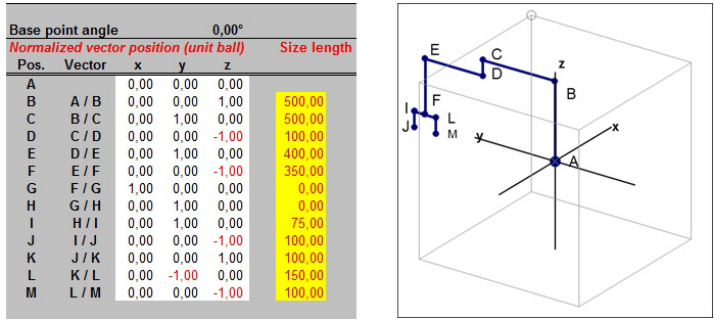
SCARA (Selective Compliance Assembly Robot Arm) are structurally sim- pler than articulated arm robots. They are usually designed as 4-axis robots. In a jointed-arm / swivel-arm robot, the B/C axis usually describes a (hori- zontal) rotary axis, C/D a rigid swivel arm. In the SCARA vice versa. The calculation for the algorithm described here is determined by the modeling per Normalized Vector Orientation, pl. see Fig. 3.
Figure 3: SCARA with ball joint (vector F/G | G/H) & End-Effector (vector H/I to L/M).
SCARA constructions differ by the “stacking direction”of their horizontal swivel arms; in the Normalized Vector Orientation this is taken into account as +/−sign (in the example C/D), all other vector positions remain the same. In the example of Fig. 3, the table area H/I to L/M models a 3D-orientable end effector (movable gripper) – by using opposing vectors. The gripper is oriented with the degree of freedom of a ball joint (vectors F/G and G/H). Fig. 3 shows the home position of the end effector oriented parallel to the swivel arms, for a transverse orientation the x and y values of the vectors H/I to L/M have to be swapped.
168 Brodtmann and Schilberg
In mechanical reality, a kinematic robot arm chain similar to Fig. 2/3 con- sists of a sequence of rotary joint, swivel arm, rotary joint, swivel arm, etc. In mechanical zero position, the swivel arms of even index number as well as the odd index number are each in a parallel alignment. The rotary joints are orthogonal to this; from the kinematic point of view of the motion chain, they are oriented antiparallel. If this parallel system is placed parallel to a ref- erence coordinate, the Normalized Vector Orientations describe the effective course of the kinematic chain in the integer 0|1|0 system. The orientation of each link of the kinematic chain, independent of whether it is a rotation axis or a swivel arm, is defined in this 0|1|0 system. Herewith the basic structure of the kinematic chain is completely modeled.
The rotation matrices [2_02] transform the Normalized Vector Orien- tation into individual vectors of the unit sphere cascade, with which the real construction dimension of each chain link is scaled. This results in a zero point related vector orientation for each chain link. The addition of this vector orientation models the real position of the robot links in a 3 dimensional space. Telescope arms - i.e., arms of variable length - become cal- culable with individually variable size-length value. The Normalized Vector Orientation is the starting value of the kinematic chain.
Ball-/Spherical Joints The combination of Normalized Vector Orientation and R3 Rotation Matri- ces introduced into robotics in this work not only allows the kinematic calculation of orthogonally aligned rotary joints and swivel axes. The algo- rithm also handles spherical joints; the rotation axis or movement can therefore be oriented arbitrarily in the 3 dimensional space. The Normalized Vector Orientation defines the orientation for this not only in the integer 0|1|0 system: Each unit sphere describes with radius 1 the vector position in the Cartesian (world) Coordinate Reference System (CRS) respectively CCR related to the reference point 0|0|0.
The Geographical Coordinate System describes the position of a point on the sphere by means of longitude (ϕ) and latitude (θ). Longitudes are defined as great circles, latitudes as small circles. Considering the elevation angle of the Cartesian system as the latitude of the Geographic system, the elevation angle defines a small circle whose periphery is locus of the sphere vector. In the unit sphere, the xyz vectors are calculated following polar coordinates (by swapped sin/cos relation θ): Vector component “x” = cos (θ) * cos (ϕ) Vector component “y” = cos (θ) * sin (ϕ) Vector component “z” = sin (θ)
Parameterization The consequent separation of motion calculation by rotation matrices and mechanical modeling by Normalized Vector Orientation - combined with a matrix independent vector scaling to real construction dimensions - enables,
Kinematics of Serial Robotics Algorithms for Simplified Calculation 169
to calculate orientations with component size “0” (zero). Several rotary axes of arbitrary orientation can be mapped together in one point. -This corresponds to the degree of freedom of a ball joint (Fig. 3 FG / GH).
a holistic, flexible base point algorithm: Robot designs differ in the base point area whether the vertical (main) rotary axis and the first horizontal rotary axis are intersecting (Fig. 1 a) or lie next to each other with a xy position of B different to A (Fig. 1 b). If the horizontal axis of rotation is adjacent to the vertical axis of rota- tion, the axes do not intersect. With relation to the base point 0|0|0, the axis offset in the unit sphere system is interpreted as a vector skew, which defines a small circle of the sphere. Independent of the horizontal axis off- set, the first rotation matrix of the matrix cascade always rotates around the vertical axis with base point 0|0|0. The first horizontal axis rotates with small circle offset on its periphery. For example: With a horizontal axis offset corresponding to the effective vertical height, the small circle is at 45
, parameterized per Normalized Vector Orientation 0.7071 | 0 | 0.7071. The algorithm works holistically, it does not distinguish whether the hor- izontal axis is offset or intersects with the vertical one. If this is the case, the horizontal axis rotates with small circle 90
corresponding to radius 0 centrically above the vertical one.
R3 Rotation Matrices According to Euler Prof. Dr. (Purgathofer), Geometrische Transformationen presents the basics very clearly. The matrix overview cf. [2_01] is based on his publication. According to EULER, the following 3 transformation matrices are available for the
The classical method is clear with its outward and backward rotations, but requires 6 transformation steps. The classical Eulerian rotation matri- ces consist of 3 columns and 3 rows, i.e. 9 elements; to each of which 4 angle-determining sin/cos values per rotation axis xyz are assigned. If addi- tionally homogeneous coordinates must be calculated, 4x4 = 16 elements are involved. In sum, 6 of these matrices (4 pcs. 3x3 as well as 2 pcs. 4x4) are required for the stepwise outward and backward rotation. A first one (4x4) for the parallel vector transfer in zero position, 2 for the rotation in calcula- tion position, 1 for the desired rotation around the transferred spatial axis, 2 for the back rotation including the xyz offset by means of homogeneous coordinates. In total, about 180 multiplications and additions are required.
170 Brodtmann and Schilberg
R3 Rotation Matrix Much rarer than the DH conventions, a transformation algorithm can be found in literature and on the Internet, which is usually called R3 Rotation Matrix. As far as I have researched, it has not yet been introduced in robotics by now. This 3x3 matrix summarizes the functionality of the described 6 single transformation steps. The vector calculation by unit sphere makes it possible to do without homogeneous coordinates, in addition multiplica- tions and divisions “with 1” are omitted; matrix results and scalar product etc. become trigonometrically directly evaluable. Although each of the 9 ele- ments consists on average of 4 multiplications plus one addition, the matrix multiplications (compared to the classical approach according to [2_01]) are reduced by a factor of about 6.
Source Citation and Derivation
Emslander, Lotte (2009), Rotationen im R3, student research project. Prof. Dr. Martin Schmidt, Universität Mannheim.
Kern Thomas, (1998) Grundlegende mathematische Verfahren der 3D- Visualisierung, student research project. Prof. Dr.-Ing. habil. H. Rothe, Universität der Bundeswehr, Hamburg, Institut für Automatisierung- stechnik.
The matrix can also be found in a similar form at https://de.wikipedia. org/wiki /Drehmatrix.
Matrices Building Blocks The orientation of an input vector x|y|z is transferred by the opera- tional rotation angle α into an output vector. Whether these vector describe a rotation axis or a swivel arm is determined by the parame- terization via Normalized Vector Orientation (cf. Fig. 2/3). This allows universal, unlimited cascadable matrix blocks. Each building block con- sists of the R3 rotation matrix and the transformed (remaining) vector packet.
Input variables are - external the construction length of the corresponding chain link and its current angle of rotation, - internal the unit sphere output values of the predecessor matrix. The first matrix in the cascade receives its input values from the Normalized Vector Orientation.
Kinematics of Serial Robotics Algorithms for Simplified Calculation 171
Output values are - externally the construction length determined “real” space point posi- tion of the building block corresponding arm segment, - internally the transferred unit vectors of the remaining kinematic chain – which are Input of the following stage.
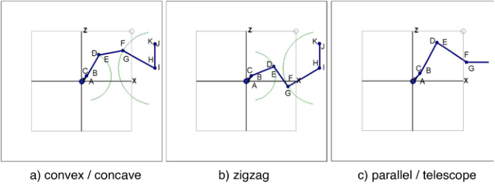
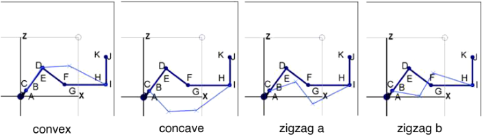
Figure 4: a) Convex / concave, b) zigzag, and c) parallel / telescope.
From cascade level to cascade level the ball chain index as well as the num- ber of vectors to be transformed is reduced by “1”. The remaining ball chain and vectors move up, therefore identical blocks can be used for the whole cascade. Each block of the cascade calculates the real space point position of its corresponding hardware link. For this purpose, the xyz vectors of the (upwardly shifted) very first unit sphere of the block will scale the position and orientation of the hardware in Vector orientation of 3D space - according to the real dimensions. The algorithm works zero-point related in the consis- tent Coordinate Reference System (CRS), thus the real 3D space points are vectorially directly addable.
CONCLUSION
The algorithms presented here master kinematic degrees of freedom of a robot mechanics beyond the (published) known extent, which is additionally twistable in itself (similar to a human upper or lower arm). Joints and arm segments can take over functions alternately; they do not have to stand perpendicularly “rigidly” on each other like in classical robot mechanics. Spherical joints become computable. Last but not least. The Normalized Vec- tor Orientation in connection with the R3 Rotation Matrices introduced here in robotics allow a doubtless and clear parameter assignment without any risk of confusion.
Direct & Inverse Kinematics The R3 rotation matrices output the kink points of the kinematic chain as vectors octant conform,
in Direct Kinematics vector values are obtained from the given angles,
in Inverse Kinematics the rotation angles of the robot system are calculated from this.
172 Brodtmann and Schilberg
The inverse kinematics presented here works with catch / snapping algo- rithms of iterative approximation. This approach is being made possible by the relatively new PC technology. Approximations are no longer “inaccu- rate”; approximations reach error deviations in the order of < 10-6 to 10-9 in msec.
Kinematics Classification The definitional distinction introduced here between a mechanics-oriented parallel-plane versus an oblique planar kinematics in addition to the (classi- cal) distinction between Direct and Inverse Kinematics is not yet established in the literature, however, it makes sense in the focus of inverse kinematics. In parallel-plane kinematics, all arm segments move in parallel planes, their joints are orthogonal to this, also parallel. Inverse parallel-plane kinematics is 2-dimensional computable.
If swivel arms are given the additional degree of freedom of an integrated rotary axis, the rotary axes and the swivel arms do not move in parallel planes but obliquely on each other, which has given the term Oblique-plane Kine- matics. The degree of freedom of this kinematics corresponds to human upper and lower arms. The term Oblique-plane Kinematic is linguistically derived from the mathematical term of the oblique joint, the inclined or oblique plane, etc.
For the snapping algorithms of Inverse Oblique Plane Kinematics, each “Forward” brick calculates with “its” R3 rotation matrix the start coordi- nates of a kinematic backward chain step by step. In a similar block cascade as described above, an additional block cascade using end effector’s / TCP target position as starting point calculates each arm and joint position in “Forward Kinematics backward”. Both kinematic chains work in the same Coordinate Reference System (CRS), corresponding point positions in 3D space allow catch algorithms of the inverse oblique-plane kinematics. How- ever, the snapping algorithms has to be calculated 3-dimensionally - with a considerably higher computational effort.
Due to the limited place of this paper, only snapping algorithms of inverse parallel-plane kinematics are described here. Inverse oblique plane kinemat- ics can be modeled in a similar philosophy. The philosophy of both catch processes is to virtually split the robot arm into 2 parts which “catch” each other. The kinematic chain begins (starts) in the definitions chosen here in point “A” and ends in the target point. In analogy
the arm part calculated from the start point “A” of the kinematic chain is called start arm,
the arm part starting at the target point is called target arm.
The spatial points of the kinks are marked with the letters A/B/C/... /L/M. This nomenclature refers to the start arm, the corresponding points of the target arm have the designations M’/L’/... / C’/B’/A’ in the corresponding “backwards counting method”. According to the kinematic chain an arm seg- ment D/E of the start arm thus receives the corresponding vector designation E’/D’ in the target arm.
Kinematics of Serial Robotics Algorithms for Simplified Calculation 173
Inverse Parallel Plane Kinematics The motion vector of the target point is initially transferred to all arm points of the target arm part in parallel, the target arm part is thus displaced in parallel. This creates a gap between corresponding start arm and target arm points. The “middle” arm segments catch each other to close this gap. The method strategically limits the theoretically infinite variety of solutions:
By parameterizing “how which”arm segments have to move during catch- ing, it is clearly determinable which “silhouette” the arm segments form in target position.
The danger of uncontrolled singularity is thereby systemically avoided.
For Inverse Parallel Plane Kinematics, the strategies or silhouettes are currently implemented in the simulation (cf. Fig. 4/5): Semi-Automatic: Precise roughly manual angle preselection from Direct Kinematics “in similar silhouette” (deviation < 10-5). Convex: The middle arm element lies above the target point, Concave, works vice versa to convex Zigzag a/b: The arm elements form two possible zigzag silhouettes Parallel, moves the ‘end-effector’ parallel to itself. Telescope, moves the ‘end-effector’ as if on a “telescopic extension”.
According to different hardware constructions, the swivel arm “G/H” is followed in kinematic chain either by another independent swivel arm “I/J” or by the “wrist” leading the end effector. For the snapping processes convex, concave, zigzag the effective length between the point G’ and the correspond- ing “parallel” rotation axis of the target arm, - which catches in “forward kinematics backwards”-, is dimensionally determinative.
Strategies Convex, Concave, Zigzag a/b In the examples, - strategy independent - the arm element I/J is always ori- ented the same way. It symbolizes the end effector (TCP) in this figures. If the movement strategy is maintained, I/J moves according to the target offset. If the strategies are changed, this is coupled with an undefined extension of the arm beyond the target point, which can lead to an extraneous collision.
Figure 5: The arm elements lying in parallel planes are displayed together in one drawing plane.
174 Brodtmann and Schilberg
The examples Fig. 4 show the arm silhouette already known from the per- spective view according to Fig. 1 in a 2D plan projection transferred to the first quadrant. The alternative silhouettes resulting from the motion strategies are shown in blue.
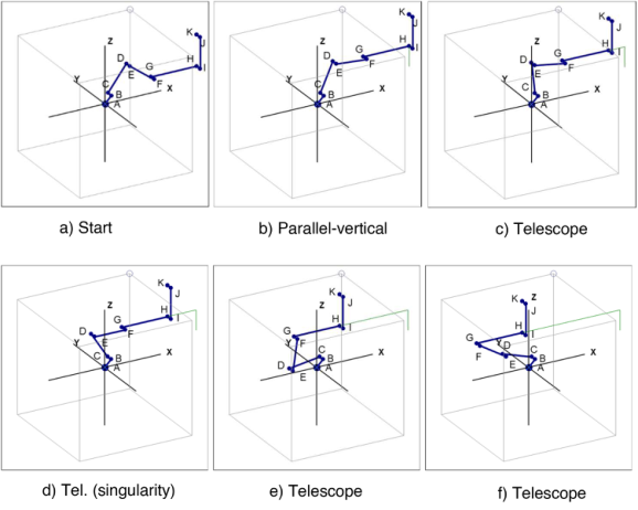
Strategies Parallel & Telescope The arm element “G/H” is pre-positioned according to the motion offset, it remains stationary during the catching process (Fig. 5).
Fig. 5 shows linear movements of the TCP from rotational movements of the axes. For the sake of clarity, these are shown here with simple movements parallel to the coordinate system.
The point H (green) draws a linear path/track.
- Strategy Parallel moves arm G/H with I/J parallel, (Fig. 5b) - Strategy Telescope moves point H in orientation G/H collinear, (Fig. 5c to f) in Fig. 5d) the axes D/E and F/G (arm E/F) pass through the singularity point.
Figure 6: a) Start. b) Parallel-vertical. c) Telescope. d) Tel. (singularity). e) Telescope. f) Telescope.
Strategy Semi-Automatic The target position roughly pre-selected in the desired orientation “by hand” using Direct Kinematics will be specified in Inverse Kinematics to the carte- sian target coordinates without changing the silhouette. Free orientation of the TCP “by hand” to any target coordinates is thus possible.
Snap Process For the calculation, the arm is first transformed “to zero” from any quad- rant around the z-axis. All swivel arm planes are now parallel to the
Kinematics of Serial Robotics Algorithms for Simplified Calculation 175 x-coordinate, so that the calculation of the snapping process can be done 2-dimensionally.The perspective (cf. Fig. 1 to 5) can be displayed in a uni- form projection plane. The aim and the general rule for all strategies is to move the peripheral points of radius C/D and H’/G’ towards or away from each other in a reproducible movement pattern and to choose the “arm length E/F” as the reference control. The transformed set points are target values of the snap process. After its completion, the gap between start arm and target arm of all corresponding points resulting from the motion off- set of the TCP is closed. The absolute coordinates of the kink points are defined in the 3D space, the angle values of the arms can be calculated from this.
Iterative Snapping For the strategies convex, concave, zigzag the swivel arms C/D and H’/G’ each describe a circle with the radius of their lengths (cf. Fig. 6 a/b). Segment areas of these two peripheries can be connected with a distance of the arm length E/F. Outside this range of validity there is no solution, inside there is also the problem of an infinite number of solutions.
For the iterative snap movement, swivel arm C/D rotate around rotat- ing axis B/C and swivel arm H’/G’ around rotating axis I’/H’ until the distance “D” to “G” corresponds to the arm length E/F.
The start position of C/D or H’/G’ and the ratio of the angular velocities B/C to I’/H’ determine the silhouette of the catch result, - an additional determination of peripheral validity areas is not necessary. - The snapping strategy avoids uncontrolled singularity.
If the starting positions and angular velocity are kept the same while the target values change, continuously moving arm silhouettes will result according to the selected strategy.
Danger of collision If the strategy and thus silhouette is changed, this leads from kine- matically uncalculated stretching of the arm into an uncontrolled path movement of the TCP / end effector.
For the strategies parallel and telescope, the arm element G/H is pre- positioned according to the motion offset, it remains stationary during the snapping process; the snapping motion is performed from swivel arm C/D only.
Special Case SCARA With SCARA, no snapping process is required. The restricted degree of free- dom makes it possible to directly calculate the swivel arm positions “in top view” 2-D trigonometrically. A Self-collision risk exists between the first swivel arm and the vertical stroke axis.
SUMMARY The mathematics of Direct and Inverse kinematics published here for the first time shows different solutions compared with the robot literature named in the bibliography and reference list. In order to be able to judge the degree of
176 Brodtmann and Schilberg
innovation of my solution, I have searched intensively in the internet, but I did not find comparable simple solutions. This is especially true for inverse kinematics, where the problem is intensively studied, but solutions are given only rudimentarily.
Only in the works of [Husty] and [Groh] target-oriented solution approaches could be found, which are based on polynomials of the 16th degree. These are also considered by the authors to be mathematically complex and are further developed with the aim of simplification.
The algorithms published are available as a Mathematical 3D Joint Construction kit - Simulation for R & T –axes realized under EXCEL®. The algorithms allow a 3D motion simulation of the robot arm move- ments as well as the end effector’s path of motion. For a video cf. also: https://www.youtube.com/watch?v=MJbAxZ3Iuio.
The kinematic calculations are visualized in real-time simulation with freely selectable perspective. For hardware control, in addition a motion protocol is output via data file.
The algorithms of Inverse parallel plane kinematics achieve – related to a stretched robot arm length about 1500 mm – TCP path deviation tar- get/actual < 10-5 mm. This development step is completed, the algorithms work stable.
In ß development phase is the also published solution approach of Inverse Oblique Plane Kinematics.
The figures used here were generated and rendered with the simulation. More info: www.RoBo-mac.de.
ACKNOWLEDGMENT
The author would like to acknowledge Dr. rer. nat. Thomas Harbich for our intensive discussions and his useful hints.
REFERENCES
Print Kreuzer, E. J. (1994) Prof. Dr.-Ing., Dr.-Ing. J.-B. Lugtenburg, Dr.-Ing. H.-G.
Meißner, Dr.-Ing. A. Truckenbrodt, Industrieroboter / Technik, Berechnung u. anwendungsorientierte Auslegung. Springer 1094 ISBN 978-3-642-93508-4. Waldron (2016), Kenneth J. Prof. Ph.D. University of Technology Sydney, Australia / Schmiedeler (2016), James, Prof. Ph.D. University of Notre Dame, Handbook of Robotics Springer ISBN: 978-3-319-32550-7 DOI 10.1007/978-3-319-32552-1 Weber, Wolfgang (2009/2013) Prof. Dr.-Ing. Industrieroboter, Methoden der
Steuerung und Regelung. Carl Hanser Verlag, München Wien, 2009, ISBN 978-3-446-41031-2.
Internet/Online Lecture Asfour, Tamin Prof. Dr.-Ing. / Dr.-Ing. Peter Kaiser Direkte und Inverse Kinematik, Denavit-Hartenberg Konvention, Jacobi-Matrizen. Karlsruher Institut of Tech- nologies (KIT), https://www.youtube.com/watch?v=8FdBSGSRCmY https://ww w.youtube.com/watch?v=uKIHRZe8O60
Kinematics of Serial Robotics Algorithms for Simplified Calculation 177
Emslander, Lotte (2009), Rotationen im R3, student research project. Prof.
Dr. Martin Schmidt, University of Mannheim, Chair of Geometric Anal- ysis, http://analysis.math.uni-mannheim.de/lehre/fs09/anageo/uebung/unsichtbar /Rotationen_im_R3.pdf No longer online, Paper copy archived here with refer- encing permission by Prof. Dr. Schmidt. Funk, Gerhard Univ. Prof. Dr. Digital Media for Artists. Universität f. künstlerische u. industrielle Gestaltung, Linz http://www.dma.ufg.ac.at/app/link/Grundlagen% 3A3D-Grafik/module/9320?step=all#chapter Globke, Wolfgang Dipl.-Inform., Koordinaten; Transformation und Roboter. Präsentation Karlsruher Institut of Technologies (KIT). Institut für Algebra und Geometrie https://www.math.kit.edu/iag2/~globke/media/koordinaten.pdf Groh, Friedemann Dipl.-Phys., Dissertation Numerische Verfahren für Polynomsys-
teme mit Anwendungen in der Robotik (2014) https://elib.uni-stuttgart.de/bitstr eam/11682/4629/1/Groh_42.pdf Henrich, Dominik, Diplom-Arbeit, On-line Kollisionserkennung mit hierarchisch modellierten Hindernissen für ein Mehrarm-Robotersystem. Technische Uni- versität Kaiserslautern https://kluedo.ub.uni-kl.de/frontdoor/index/index/docId/ 1029 Husty, Manfred Univ.-Prof. Dr. Dr.h.c., Implementierung eines neuartigen, effizien-
ten Algorithmus zur Berechnung der inversen Kinematik von seriellen Robotern mit Drehgelenken. Universität Innsbruck http://geometrie.uibk.ac.at/cms/datasto re/husty/husty-linz.pdf Kern, Thomas, (1998) Grundlegende mathematische Verfahren der 3D- Visualisierung, student research project. Prof. Dr.-Ing. habil. H. Rothe, Universität der Bundeswehr, Hamburg, Institut für Automatisierungstechnik No longer online, Paper copy archived here with referencing permission by Prof. Dr. Rothe. Kern, 3D-Visualisierung / Rotationsmatrix http://www.3dsource.de/deutsch/3Dma the.htm http://www.3dsource.de/_download/Anhang_Rotation.pdf Pope, Andy, Website AJP Excel Infortion.
3D-Rotation http://www.andypope.info/charts/3drotate.htm Excel® Special https://andypope.info/charts.htm Preim, Bernhard Prof. Dr.-Ing. habil., Universität Magdeburg Planare Projektionen und Betrachtungstransformation. http://isgwww.cs.uni-magdeburg.de/~ber nhard/cg/vorl6Projektionen.pdf Purgathofer, Werner Univ.-Prof. Dipl.-Ing. Dr. techn. Dr.h.c., Geometrische Transfor-
mationen. TU Wien https://www.cg.tuwien.ac.at/courses/CG1/textblaetter/02% 20Geometrische%20Transformationen.pdf Thiele, Stephan, Architekt Raumsprache, Handbuch zur Architekturskizze. www.thiele-architekt.de/pdf/Raumsprache-A5.pdf (nicht mehr Online, archiviert). Excerpt https://www.tilp-wn.de/mphif/zentproj.htm Wüst, Klaus Prof. Dr. Grundlagen der Robotik / Festlegung der Koordinatensysteme / Transformationen der Koordinatensysteme / Parameter aus den Transformationen. TH Mittelhessen https://homepages.thm.de/~hg6458/Robotik/Robotik.pdf https://homepages.thm.de/~hg6458/Robotik/Denavit-Hartenberg.pdf https://homepages.thm.de/~hg6458/ROB_ERG.pdf Ziya, ¸Sanal, (2015) Prof., Mathematik für Ingenieure, 6.1 Koordinatensysteme.
Türkisch-Deutsche Universität, Istanbul DOI: 10.1007/978-3-658-10642-3_6, https://link.springer.com/chapter/10.1007%2F978-3-658-10642-3_6
LISTED IN THE AHFE DIGITAL BOOKSTORE CATALOGUE
Explore the complete digital volume
Emerging Technologies and Future of Work
Read this individual research paper free through the original publisher, or explore the full digital proceedings book.
ISBN 978-1-958651-93-3
Explore this ISBN in the AHFE Bookstore ↗Listed in the July 2026 bookstore catalogue; search by ISBN to confirm current availability · Digital book purchase optional