Wang Jianlun, Deng Huangtianci, Su Rina, Can He, Han Yu, He Jianlei, Hu Baoyue, Chen Husheng, Huang Sheng, Xiao Sirong, Cao Jinduo (2023). A sample-based method of 3D reconstruction for plant leaf from single image or multiple images. In: Artificial Intelligence, Social Computing and Wearable Technologies. AHFE Open Access, vol. 113, pp. 226–237. https://doi.org/10.54941/ahfe1004195
Agricultural operations require simple, efficient and robust measurement method of three dimensional forms for the plant organs such as leaves to analyse other kinds of phenotype in detail on this basis. However, most of the existing sample-based methods reconstruct three dimensional shapes of the images for the objects of smooth surface and homogeneous materials, such as plastics, paints, ceramics, and metals, etc., rather than for the natural objects of convex-concave surfaces and varying albedo materials under the arbitrary natural lights. In this paper, it was found that the methods based on the prior model with photometric stereo superposed BRDF proposed can accurately realize the 3D modelling for plant leaf image and may reduce the cumulative error. With the differential gradient constraint and integral gradient constraint proposed, the unique solution for the normal vectors of all micro panels of the pixel projection on the leaf surface was matched by the first-order central difference equation and the iterations, and this process solved the ill-posed problem of BRDF. The experiment results showed that the average error between the height reconstructed results and the measured results of the real leaves’ height was 15% and the attenuation error was reduced by our method.
Understanding the three-dimensional (3D) shape and the texture of a plant leaf is one of the important means to monitor agricultural production. Shadow is an important depth cue in human vision, on this bases many approaches were proceeded (Horn, 1986).
Photometric Stereo provides a method to determine the surface normal vector for the anisotropic and non-Lambertian material (Woodham, 1980) by changing the angle and the direction of incident lights between succes- sive images and keeping the observation direction unchanged, in the process,
A Sample-Based Method of 3D Reconstruction for Plant Leaf From Single Image 227
the incident light directions should be calibrated. Some approaches of pho- tometric stereo match the multidimensional vector of the reflected radiance and search for the surface normal vector in the prior model to avoid the cali- bration of the incident light directions (Woodham, 1994). Photometric stereo method is valid when the sample material of the model is exactly the same as that of the reconstructed object in a particular shape, and both of them are homogeneous (Silver, 1980). BRDF is convenient to derive the normal vectors of the object surface under a fixed scene illumination from a single model, but the micro facet of the pixel projection on the surface of the object has two degrees of freedom so that it leads to an ill-posed problem in solving the surface normal vector (Torrance et al. 1967). Usually the function is not used alone to rebuild shape from shading, a prior model and other constraints are needed. In the existing literature, the materials of the image reconstructed objects used in the prior model are mostly plastics, ceramics, paints and metals etc., they are all smooth or at least homogeneous (Logothetis et al. 2023). When some error factors are so small that can be ignored, the normal vector of the surface of the object can be easily and accurately obtained by these matching algorithms, as K nearest neighbour method (Hertzmann et al. 2005), Convolutional neural network (Kaya1, 2021), etc. The situations are more complicated in solving the normal vector of the natural objects surface, such as plant leaves in reality. On the one hand, the plant leaves generally appear to have relatively homogeneous material, but there are veins, stomata, villus and waxy covering layer and other fine structures throughout the surface. These tiny structures make the leaves not absolutely homogeneous and not strictly isotropic. Plant leaves are also not considered as the standard Lambert body. It is difficult to accurately match the multidimensional vectors of the reflected radiance between a prior model and an object leaf to search the exact surface normal vector. However, on the other hand, the leaves of plants are not always very smooth, there are subtle or local convex-concave phenomena, one-to-one matching the multidimen- sional vectors of the reflected radiance to search normal vector is susceptible to the noises of the geometrical attenuations. Under these circumstances, the mapping between the reflected radiance and surface normal vector for the prior model will be somewhat different to that for the reconstructed plant leaf. Meanwhile the non-local reflections may also cause noise interference. All of these can lead to accumulated errors in height integration caused by the mismatching.
Still, the following assumptions need to be established in the reconstruction:
The plant leaf surface is assumed to be continuously differentiable, so that the differential gradient of the normal vectors between the neighbour pixels can be obtained.
The plant leaves are assumed to be homogeneous, the normal vector direction angles of the surface can map the reflected radiance.
Assuming the image taken by the camera is orthogonal projection, 3D coordinates can be established on the plane of the plant leaf image.
The reference and the object leaves are under the same lighting conditions, BRDF of the object lies within the linear span of that of the reference.
This paper introduced Photometric Stereo superposition method into BRDF. The raw data of the normal vector direction angles and the superposed reflected radiance of the overlaid sample images on the reference hemisphere surface were obtained. After that the prior model was built by the supervised learning. With this prior model, two solutions of the gradients between the direction angles of two adjacent micro surfaces were acquired by the gradi- ent differential constraint, and then two solutions of the normal direction angles of the micro surfaces for the adjacent pixels were solved by the gra- dient integral constraint. The reintegration process is dovish and can reduce the errors from geometrical attenuation and subtle non-homogeneous. Then, by using the first-order central difference equation, the unique solution of the four-neighbourhood normal vectors is solved by substituting the combined solutions of the four-neighbourhood pixels into the equation respectively. The height modelling is based on the iteration method.
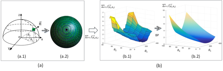
INVERSE PHOTOMETRIC STEREO PRIOR MODEL BRDF expresses the relationship between the surface albedo and the normal vector, while the orientation consistency principle indicates that the normal vector of the micro facets with the same albedos are the same under the same illumination. Using the hemisphere covered by plant leaf samples as the ref- erence model, the relationship between the normal direction angles and the grayscale of the surface can be established (See Figure 1(a.1)).
Figure 1: Schematic of the prior model of photometric stereo superposition. (a) Rela- tionship between the normal direction angles and the grayscale on a hemisphere. (a.1) The normal vector of the reference hemisphere surface. (a. 2) The reference hemi- sphere of the plant leaf samples. (b) The prior model of normal direction angles and superposed grayscales. (b.1) The raw data set. (b.2) The data set learned by BP neural network.
The function of the reflection at each micro facet of the pixel projection under a given incident light is as follows:
f i
Equations and mathematical formulas are available in the original paper PDF.
A Sample-Based Method of 3D Reconstruction for Plant Leaf From Single Image 229 Under an incident light i whose unit vector is −→s i and intensity is Li, all the reflected radiances are normalized by a maximum grayscale in an image range. And the grayscales are superposed at a same pixel for all of the images shot under the different incident lights, as shown in the following formula:
[Equation or mathematical symbol available in the original paper PDF]
[Equation or mathematical symbol available in the original paper PDF]
f i
n X
n X
[Equation or mathematical symbol available in the original paper PDF]
The function (1) of the reflection is substituted into the formula (2) to obtain the discrete reflected radiance of the superposition:
n X
n X
n X
ρ(x,y),0 · −→ n (x,y),0 · −→s i
(θ1,θ2) (3)
i = 1 The superposed grayscale of a micro panel of the pixel projection is only related to the albedo, normal vector and unit vector of the incident light, but not the intensity of the incident light which should be uniform for the single image.
x, y
Where (θ1, θ2) are the normal direction angles,
are the pixel coor- dinates, −→ n (x,y) is the normal vector of the micro facets of the leaf, the Pn
Equations and mathematical formulas are available in the original paper PDF.
(θ1,θ2) are the superposed grayscale of the micro facets of the pixel projections. In a sight line, ρ(x,y),0 is the ratio of the albedo of the micro facet of the pixel
x, y
to the albedo of the micro facet of the pixel with the maximum grayscale in an image range. −→ n (x,y),0 is the nor- mal vector of the micro plane of the pixel projection and −→s i is an incident light unit vector, in the 3D coordinate system that is established on the image plane by taking the centre point of the pixel of the maximum grayscale in the rebuilding leaf area as the origin and setting the Z axis according to the right-hand rule (See Figure 4 (a)).
After superposing the reflected radiance, a data set of reference is built (See Figure 1(b.1)), and an inverted mapping is learned by BP neural network as (θ1, θ2) →Pn
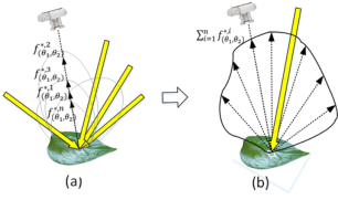
(θ1,θ2). The new data set is a curved surface looked like a univalent hyperbolic no rotational surface (See Figure 1 (b.2)). The mapping of an object leaf is supposed to be the same as that of a reference hemisphere (See Figure 1(a.2) and Figure 2 (a) and (b)).
Figure 2: Schematic diagram of the reflected radiance of the superposition on the plant leaf surface. (a) The reflected radiances of the different incident lights. (b) The superposed reflected radiance.
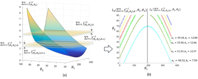
DIFFERENTIAL CONSTRAINT AND INTEGRAL CONSTRAINT OF GRADIENT Through analysis, it is found that the cross-sections of the curved surface of the data set at different grayscale points are the data lines of the two nor- mal direction angles conforming to the function J (θ1, θ2) = θ2 −a0 −
eiθ2c1 −1
e
a1 + b1
a1 −b1 i i
1 2
2
′(Pn
and RMSEs < 0.5, and a0, a1, b1, c1 are variables on the curved surface (See Figure 3(a)). When b1 ≪a1, the data lines will be approximate catenary lines. Cause one θ1 correspond to two θ2, the prior data set can be divided into two data sets, Lk(Pn
(θ1,θ2),k + j, θ1, θ2) and Lk
(θ1,θ2),k, θ1, θ2), the left and right sides have different features. The two different curved lines of the adjacent pixels are parallel on the same side, as Lk (θ1, θ2) ∥Lk + j (θ1, θ2) and Lk
′ (θ1, θ2) ∥Lk + j
′ (θ1, θ2) (See Figure 3(b)). Because the gradients of the normal direction angles for the adjacent micro facets are approximately equal between the two curves on the same side, the two different gradients of each direction angle can be obtained respectively on each side of the lines, as (1θ1, 1θ2) and (1θ1, 1θ2)′.
! ,
! ,
The two differential constrains of the gradient on the two sides of the curved lines are as follows:
Pmk
Pmk + j mk
mk + j
1θ1
1θ2
k,k + j
1 1 θLk
2 1 θ
Lk + j 1
! ,
! ,
Pmk
Pmk + j mk
mk + j
1 1 θLk
2 1 θ
Lk + j 2
and
Equations and mathematical formulas are available in the original paper PDF.
, , L′ ′
mk + j mk
1θ1
1θ2
k + j 1 k 1
k,k + j
k,k + j
Equations and mathematical formulas are available in the original paper PDF.
1 θ
1 θ
Equations and mathematical formulas are available in the original paper PDF.
, , L′
mk + j mk 2 −
2 (4)
k + j 2 k 2 [Equation or mathematical symbol available in the original paper PDF]
[Equation or mathematical symbol available in the original paper PDF]
Equations and mathematical formulas are available in the original paper PDF.
1 θ
1 θ
Then the two solutions of the normal direction angles of the adjacent micro panels of the pixel projections are as follows: θk + j
1θ1
1θ2
1 +
2 +
k,k + j , θk + j
Equations and mathematical formulas are available in the original paper PDF.
θk
θk + j
θk + j
θk
1θ1 ′
1θ2 ′
1 ′
2 ′
1 ′
2 ′
k,k + j
k,k + j ,
Where mk
1, mk 2 and mk + j 1 , mk + j
2 , are the number of the data of
θk
θk
θk + 1
θk + 1
respectively. And
and
1, θk 2
1, θk 2 ′
1 , θk + 1
2
1 , θk + 1
2 ′
j = 1, 2, 3, 4 is the ordinal number arranged in the descending order of the grayscales of the four neighbourhood pixels for a central pixel.
Starting from the panel of the pixel projection with the highest grayscale in the leaf area, the gradients of the normal direction angles are calculated
A Sample-Based Method of 3D Reconstruction for Plant Leaf From Single Image 231
for the adjacent panels of the four-neighbourhoods in the descending order of the grayscales, the solutions of the normal direction angles for all of the micro panels in the reconstruction region can be obtained by the following integrations: θk + j
1θ1
1θ1
1θ1
1
1 + R m
m d
Equations and mathematical formulas are available in the original paper PDF.
θk + j
1θ2
1θ2
1θ2
1
2 + R m
m d
Equations and mathematical formulas are available in the original paper PDF.
′,
1θ1 ′
1θ1 ′ +
1θ1
1 + Z m
1 ′
md
k,k + j
θk + j
′ (6)
1θ2 ′ d
1θ2 ′ +
1θ2
2 + Z m
2 ′
k,k + j
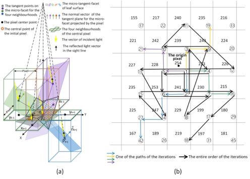
Where m is the length variable of the paths of the iterations starting from the initial pixel to an arbitrary central pixel k (See Figure 4(b)). Then the two normal vector solutions for each four-neighbourhood micro facet can be obtained.
Figure 3: Schematic diagram of the gradient differential constraint: (a) The curved sur- face of the two normal direction angles and the superimposed grayscales. (b) The gradients of the two normal direction angels between the two cross-section lines of the adjacent pixels are approximately equal.
NEIGHBUORHOOD-CENTER DIFFERENCE METHOD AND HEIGHT ITERATION PATHS
Let −→ P k [xk, yk, zk] be the tangent point vector of the micro-surface element of a central pixel projection, and let −→ P k+j
xk+j, yk+j, zk+j
be the tangent point vector of the micro facet projected by a neighbourhood pixel. The normal vector of the neighbourhood micro panel is as follows:
#
pk+j, qk+j, −1
The point-normal equation of the neighbourhood micro facets is the follow:
−→ n k+j ·
−→ P k −−→ P k+j
When the tangent point vector −→ P k, the coordinates
xk+j, yk+j
and the normal vector −→ n k+j of the adjacent micro facet are substituted into the pointnormal equation (8), the zk+j part of the tangent point vector −→ P k+j can be obtained.
Let the normal vector of the micro facet at the origin be [0,0, −1]. For the micro facet at the origin, when the two pairs of solutions of the two normal vectors for each four-neighbourhood micro facet are obtained, 16 possible permutation of the normal vector solutions and 16 possible zk+j part of the tangent point vector −→ P k+j will also be obtained. When the micro facet is not at the origin, the number of possible solutions for the normal vectors of the four-neighbourhoods is determined by the number of the undetermined normal vectors of the neighbourhoods.
Let the normal vector [pk, qk, −1] of a central micro facet be known, and the four adjacent micro facet are marked by xk + 1, xk−1, yk + 1 and yk−1 respectively (See Figure 4(a)). The first order central difference equations are as follows:
zxk + 1
zyk + 1
k −zxk−1
k −zyk−1
k 2 ,
k 2 (9)
k
k
In this paper, up to 16 permutation solutions of the zk+j parts of the tan- gent point vectors of for the four neighbourhoods were substituted into the above formula respectively. It is verified by experiments that only one of the solutions matches the partial derivative of the central micro surface. So that the unique solution of the normal vectors −→ n k+j of the four-neighbourhood micro facets is obtained. Then the next central pixel is the pixel of the largest grayscale in the four neighbourhoods of the former central pixel. The 3D coordinates of the tangent points
xk, yk, zk
of the global micro facets of a leaf can be obtained by the chain iterations in the descending order (See Figure 4(b)).
Figure 4: Schematic of the micro structure of the four neighbourhoods and the paths of the height iterations. (a) The micro structure of the four neighbourhoods. (b) The paths of the height iterations (the data in the grids are the grayscale value of a pixel and the sequence number of the iteration order).
A Sample-Based Method of 3D Reconstruction for Plant Leaf From Single Image 233
EXPERIMENT The scindapsus aureus leaves were selected as the reconstruction objects. All images were taken from a distance of 1.67 meters at a fixed focal length under natural light in front of an indoor window. 5 mm wide arcs of the fresh leaves were affixed to the centre of the latitude lines on the outer surface of the hemisphere which was marked with the longitude and latitude lines at intervals of 10 degrees and with a radius of 100 mm. By changing the angle and direction of the incident lights between the 9 consecutive images, the images of the hemispherical reference samples and the 60 leaves were obtained (See Figure 5).
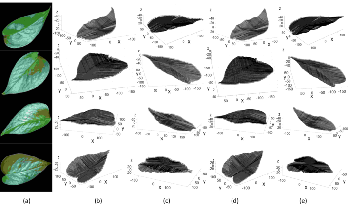
Figure 5: One of the 9 images of the plant leaves and the reference hemisphere.Figure 6: The 3d reconstruction results (coordinate units are pixels). (a) The original image of the leaves. (b)Top view of the rebuild leaves of one image. (c) Bottom view of the rebuild leaves of one image. (d)Top view of the rebuild leaves of nine images. (e)Bottom view of the rebuild leaves of nine images.
The image regions of each hemispherical model in the 9 images were taken out, the normal direction angles (θ1, θ2) and the mean grayscale of a 10 × 10 pixels piece were extracted at each intersection of the longitude line and lat- itude lines, and the coordinate system was established (See Figure 1(a.1)).
There were of 9 × 36 × 6 original reference sample points were derived (See Figure 1(a.2)) and then superposed (See Figure 1(b.1)). The prior data set was built at the angle intervals of 1 degree by supervised learning (See Figure 1(b.2)). The 60 leaves of each image were segmented into 60 inde- pendent leaf regions by using the Canny operator. The grayscales were superimposed for each pixel of each leaf of the 9 images (See Figure 2(a) and Figure 2 (b)).
The camera model used in the experiment is Leica M9, the effective pixels are 18 million, the sensor size is 35.8 * 23.9mm, and lens model is Leica SUMMICRON-N-M35mmf/2ASPH. The computer Processor is Intel Core i9-10900K @ 3.70GHz and the memory is 16 × 4GB.
The 3D rebuild of the leaf images were performed by taking the cross sections of the superposed grayscale for the adjacent pixels in the prior model, calculating the gradients, matching the normal vec- tors, and integrating the height of the micro facets by the chain itera- tions. The results of the reconstruction were satisfactory (See Figure 6 and Figure 7). The leaf reconstructions were performed with the single image and 9 images by our method, and both kinds of rebuild take 8.5 seconds in average.
RESULT DISCUSSION AND CONCLUSION In this paper, there are several aspects of this reconstruction process that need to be addressed.
(θ1,θ2),k →(θ1, θ2) based on the shadow is fuzzy,
Reverse modelling of reference samples In human vision, the comprehension clue of depth is the shade of the surface, but the mapping Pn while the inverse mapping (θ1, θ2) →Pn
(θ1,θ2),k can be the one-to-one mapping.
Data accuracy analysis The size of the matrix in the rebuild program will affect the precision of the reintegrate results. If more accurate data set is needed, the data of the prior model should be divided into several parts and be rebuilt in fine intervals part by part again.
The prior data set (θ1, θ2) →Pn
(θ1,θ2),k is a curved surface (See Figure 3(a)). The basic parameters of the curved surface shape corre- spond to the albedo of the leaf surface material (See formula (3)). Cause the anisotropic and non-homogeneous properties of the leaf are vari- ables, the cross-section lines change slightly with the curved surface shape (See Figure 3(b)). When the gradient of the energy for the adjacent pix- els becomes bigger, the shape of the two cross-section lines will differ a little more, and the error of the gradients between the two normal vec- tors may increase. However, because the leaf surface is continuous and differentiable, the differential gradients can ensure the accuracy of the reconstructions.
A Sample-Based Method of 3D Reconstruction for Plant Leaf From Single Image 235
The impact of the image number on 3D modelling results The differences in the reintegrated results between the single image processing and the nine images processing are apparent. The shape results of the nine images are more accurate, the 3D details, such as convex-concave surface and veins, are closer to the original leaves, and there are much fewer geometrical attenuation noise. (See Figure 6(a), (b), (c), (d) and (e)).
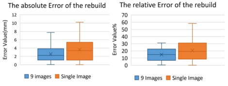
In order to verify the accuracy of the rebuilt height in pixel-scale, the real length and width of 60 object leaves were measured by coordinate paper, and the real heights of the leaves were measured by a laser measurement platform. The ratio of the real leaf length to the pixel length of the leaf image was used as the projection scale factor. The reconstructed height calculated according to the projection ratio was compared with the real leaf height, the statistical results are in tables 1 and table 2 (See Figure 7).
Table 1. The absolute errors of the rebuild results of the leaf heights.
Table available in the original PDF paper.
Type Absolute errors of 9 images Absolute errors of single image Data volume (number) 60 60 Mean value (mm) 2.5675 3.6410 Standard deviation (mm) 1.7437 2.5693 Variance 3.0406 6.6015
Table 2. The relative errors of the rebuild results of the leaf heights.
Table available in the original PDF paper.
Type Relative errors of 9 images
Relative errors of single image Data volume (number) 60 60 Mean value (%) 14.76 20.59 Standard deviation (%) 9.290 13.67 Variance 0.8641 1.871
Compared with the rebuilt results of the nine images, those of the single image had fewer original data and a faster data pre-processing speed, but lower accuracy.
The light environment factors that influence the reconstruction In this paper, the images of the object leaves and the reference samples were taken under the indoor natural light in front of the windows. While in out- door natural light environment, if the light blocking error can be reduced, the accuracy can be further improved. If the intensity distribution of the incident light is uneven in a single leaf image, or the incident lights have differences between the leaves and the reference samples of a single image, the height errors will be piled up or the reconstruction may fail. At the same time, other stray radiation from the environment entered the camera will also cause optical noise and lead to errors (See Figure 6), there are many stripe-like interference in these reintegrated 3D shapes. In the reconstruction
process, more incident lights with apparently different angles and directions could be selected to increase the rebuilding accuracy.
Figure 7: Box chart of absolute errors and relative errors of rebuild results of the leaf heights.
The experimental results show that the proposed method can be used to reconstruct the plant leaves. This method is also effective in reducing the geo- metrical attenuation error and might be used for the image reconstruction of other similar natural materials. In the future, the relation between the mate- rial albedo (Ward, 1992) and the parameters of the curved surface of the prior model could be used to help finding a more universal method to estab- lish the prior model, which may be a convenient way to carry out practical applications of the image rebuild.
ACKNOWLEDGMENT
This work was finished by our research group at China Agricultural Univer- sity. Many Master’s degree candidates in our group contributed extensively to this work.
REFERENCES
Hertzmann, Aaron and Seitz, Steven M. (2005). Example based photometric stereo: shape reconstruction with general, varying BRDFs, IEEE Transactions on Pattern Analysis and Machine Intelligence, Volume 27 No. 8. pp. 1254–1264. Horn, B. K. P. (1986) Robot Vision. New York: McGraw-Hill. Kaya1, Berk. Kumar1, Suryansh and Sarno, Francesco et al. (2021). “Neural radi-
ance fields approach to deep multi-view photometric stereo”, 2022 IEEE/CVF Winter Conference on Applications of Computer Vision (WACV), Waikoloa, HI, USA, 2022, pp. 3967–3979. Logothetis, F. Mecca, R. Budvytis, I. Cipolla, R. (2023). A CNN Based approach for the point-light photometric stereo problem, International Journal of Computer Vision Volume 131 No. 1. pp. 101–120. Silver, W. M. (1980). Determining Shape and Reflectance Using Multiple Images,
Master’s thesis, MIT, Cambridge, Mass. Torrance, K. E. Sparrow, E. M. (1967). Theory for off-specular reflection from roughened surfaces, Journal of the Optical Society of America Volume 57 No. 9, pp. 1105–1114. Ward, Gregory J. (1992). Measuring and Modelling Anisotropic Reflection. Com-
puter Graphics Volume 26 No. 2. pp. 265–272.
A Sample-Based Method of 3D Reconstruction for Plant Leaf From Single Image 237
Woodham, Robert J. (1980). Photometric method for determining surface orientation from multiple images, Optical Engineering Volume 19 Issue 1. pp. 513–531. Woodham, R. J. (1994). Gradient and Curvature from Photometric Stereo Including
Local Confidence Estimation, Journal Optical Society America Volume 11, no. 11, pp. 3050–3068.
LISTED IN THE AHFE DIGITAL BOOKSTORE CATALOGUE
Explore the complete digital volume
Artificial Intelligence, Social Computing and Wearable Technologies
Read this individual research paper free through the original publisher, or explore the full digital proceedings book.
ISBN 978-1-958651-89-6
Explore this ISBN in the AHFE Bookstore ↗Listed in the July 2026 bookstore catalogue; search by ISBN to confirm current availability · Digital book purchase optional