Andrea Gregores Coto, Andrea Fernández Martínez, Ramon Angosto Artigues, Santiago Muiños Landín, Jonathan Josue Torrez Herrera (2026). Quantifying CTGAN Training Dynamics: A Convergence-Aware Self-Adaptive Framework. In: Human Interaction and Emerging Technologies (IHIET-AI 2026): Artificial Intelligence and Future Applications. AHFE Open Access, vol. 201. https://doi.org/10.54941/ahfe1007219
Training Generative Adversarial Networks (GANs) for tabular data remains challenging due to unstable convergence between generator and discriminator. Conditional Tabular GANs (CTGANs) are particularly sensitive to hyperparameter configurations, where inadequate tuning often leads to mode collapse or degraded data fidelity. Despite existing optimization strategies, convergence is typically assessed qualitatively rather than through explicit quantitative criteria. This work introduces a convergence metric that formally characterizes adversarial training dynamics in CTGANs. The metric evaluates curve validity, stability, and decrement behavior to detect balanced generator–discriminator dynamics. It is integrated into a self-adaptive Bayesian hyperparameter optimization framework, where convergence quality and statistical data fidelity are jointly maximized through a composite objective function. The approach is validated on benchmark datasets and on a high- dimensional industrial dataset from the aluminum sector representing its potential in material science applications. Results show improved training stability and synthetic data robustness, while adaptive search space refinement reduces computational cost. The proposed methodology enables systematic, convergence- aware CTGAN training in complex real-world scenarios.
INTRODUCTION Generative Adversarial Networks (GANs) have emerged as a powerful class of models for generating high-quality synthetic data across various domains such as images, text, and structured tabular data (Goodfellow et al., 2020).
Gregores Coto, Andrea. et al. 642
In particular, Conditional Tabular GANs (CTGANs) have shown strong performance in generating tabular datasets by addressing challenges such as mixed data types, non-Gaussian and multi-modal distributions, and imbalanced categorical columns (Xu et al., 2019). These characteristics make tabular data particularly challenging, as models must capture complex dependencies while preserving statistical relationships between variables.
Despite their potential, GANs remain difficult to train due to instability in the generator–discriminator dynamics. Issues such as vanishing gradients and mode collapse can hinder convergence and limit the diversity of generated samples (Saxena & Cao, 2022a). Several approaches have been proposed to improve training stability, including architectural improvements (Saxena & Cao, 2022b), alternative objective functions such as Wasserstein GANs (Gulrajani et al., 2017), and regularization strategies like gradient penalties (Saxena & Cao, 2022). Besides, while metrics such as the proximal duality gap provide detailed insights into GAN stability (Sidheekh et al., 2021), their computational overhead limits their practical use. A key aspect of improving GAN training is hyperparameter optimization. Given the vast search space, optimization strategies based on surrogate models or Bayesian approaches can effectively balance model performance and computational cost (Dumont et al., 2022).
This study investigates the implementation of a Convergence Metric (CM) to guide the hyperparameter optimization of CTGANs on complex datasets. The proposed approach integrates Bayesian optimization with a lightweight CM, enabling efficient hyperparameter tuning while preserving high data quality.
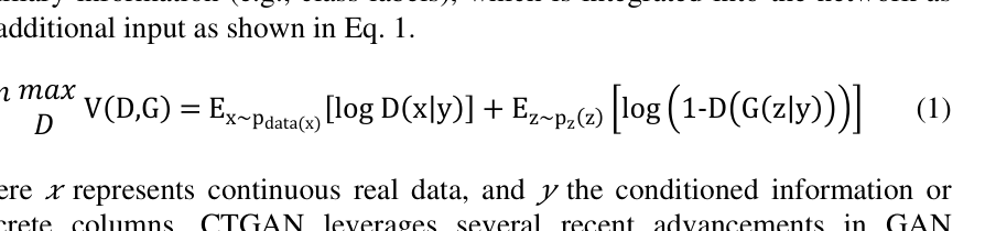
METHODOLOGY CTGAN Overview One of the advancements of CTGANs is their capability to be conditioned on auxiliary information (e.g., class labels), which is integrated into the network as an additional input as shown in Eq. 1.
𝑚𝑚𝑚𝑚𝑚𝑚
𝑚𝑚𝑚𝑚𝑚𝑚
Equation reproduced from the original PDF.
𝐺𝐺
where 𝑥𝑥 represents continuous real data, and 𝑦𝑦 the conditioned information or discrete columns. CTGAN leverages several recent advancements in GAN architectures to improve performance such as the PacGAN discriminator (Lin et al., 2018) to address mode collapse, and the WGAN-GP loss function (Gulrajani et al., 2017) to adopt the Wasserstein distance as loss function (Eq. 2).
L = EG(z) ~ Pg ൣ D൫G(z)൯ ൧−𝐸𝐸𝑥𝑥~𝑃𝑃𝑟𝑟[𝐷𝐷(𝑥𝑥)] + 𝜆𝜆𝐸𝐸𝑥𝑥ො~𝑃𝑃𝑥𝑥ෝ[(‖𝛻𝛻𝑥𝑥ො𝐷𝐷(𝑥𝑥ො)‖2 −1)2] (2) where the first two terms represent the original WGAN loss (Arjovsky et al., 2017), and the last term is a gradient penalty to regularize the discriminator. In this context, 𝑥𝑥ˆ ∼ 𝑃𝑃𝑥𝑥ˆ represents samples that are interpolated between real data
644 Gregores Coto, Andrea. et al.
𝑃𝑃𝑟𝑟 and generated data 𝑃𝑃𝑔𝑔, 𝜆𝜆 is the gradient penalty coefficient, and 𝐷𝐷(𝑥𝑥) is the discriminator function.
The architecture of the CTGAN used in this work is designed to handle the complexities of generating realistic tabular data. The generator (G) and discriminator (D) models are both optimized using the Adam optimizer. The generator employs ReLU activation in its input and hidden layers, with softmax activation for conditioned outputs and tanh activation for other outputs. The discriminator uses LeakyReLU activation in its input and hidden layers, with a sigmoid activation function at the output.
Hyperparameter Optimization Algorithm The proposed hyperparameter optimization algorithm is integrated within the Model Training component of an AI Data Pipeline (AIDP), which supports the independent development and deployment of machine learning models in industrial environments (Artigues et al., 2024). Within this framework, the component enables the self-optimization of machine learning models by automatically tuning their hyperparameters (Angosto Artigues et al., 2025). As part of this component, a self-adaptive optimization algorithm for CTGAN models is implemented using the Optuna framework (Akiba et al., 2019), which applies Bayesian optimization to iteratively refine the hyperparameter search space based on prior evaluations.
The optimization explores hyperparameters affecting both training dynamics—including learning rates, PacGAN size, and batch size—and network architecture, such as discriminator and generator dimensions. Due to computational constraints, the number of epochs is fixed at 100 across all experiments.
The algorithm employs the Tree-structured Parzen Estimator (TPE) sampler, a Bayesian optimization method that models the probability of high-performing hyperparameters based on prior trials (Watanabe, 2025). To improve efficiency, the Median Pruner terminates trials unlikely to outperform the current median based on intermediate results, reducing computational cost during GAN training.
Because GAN training is inherently stochastic, each configuration is evaluated through multiple training runs. The final score of each trial is computed as the average performance across runs, ensuring robust evaluation of candidate configurations. The optimization objective is the Overall Score (OS), which combines the Convergence Metric (CM) and the Composite Quality Metric (CQM), described in the following sections.
Convergence Metric This study introduces a Convergence Metric (CM) to evaluate CTGAN training dynamics within a self-adaptive hyperparameter optimization framework. The CM tracks generator–discriminator interactions during training and is defined in Eq. 3.
Quantifying CTGAN Training Dynamics: A Convergence-Aware Self-Adaptive Framework 645 𝐶𝐶𝐶𝐶= 𝔼𝔼ቂ𝑚𝑚𝑚𝑚𝑚𝑚ቀ0, 𝐷𝐷(𝑥𝑥𝑟𝑟𝑟𝑟𝑟𝑟𝑟𝑟) −𝐷𝐷൫𝑥𝑥𝑓𝑓𝑓𝑓𝑓𝑓𝑓𝑓൯ቁቃ (3)
Here, 𝐷𝐷(𝑥𝑥𝑟𝑟𝑟𝑟𝑟𝑟𝑟𝑟) and 𝐷𝐷൫𝑥𝑥𝑓𝑓𝑓𝑓𝑓𝑓𝑓𝑓൯ represent the discriminator’s logits for real and generated data, respectively. This metric uses the ReLU function to focus on positive differences, emphasizing instances when the generator successfully improves its performance relative to the discriminator. By filtering out negative differences, the CM reduces noise caused by temporary discriminator advantages, stabilizing the evaluation process.
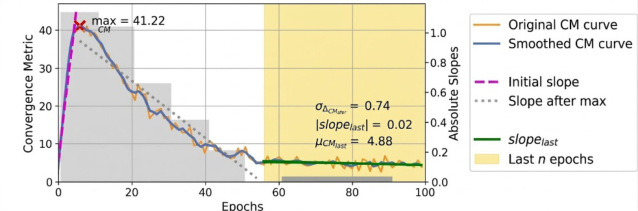
The CM curve analysis evaluates GAN convergence by assigning a score based on predefined conditions. First, the CM curve is smoothed using the Savitsky-Golay filter to reduce noise. The validity of the curve is then assessed by analyzing the balance between the generator and the discriminator (see Figure 1).
Figure 1. Example of a valid Convergence Metric (CM) curve satisfying conditions C1, C2, and C3, with stable behaviour and a clear decrement in the final training epochs.
For the CM curve to be valid, the following conditions must be satisfied:
Slope Before the Maximum: A positive slope in early epochs indicates effective discrimination between real and generated samples.
𝐶𝐶1: 𝑖𝑖𝑖𝑖𝑖𝑖𝑖𝑖𝑖𝑖𝑖𝑖𝑖𝑖 𝑠𝑠𝑠𝑠𝑠𝑠𝑠𝑠𝑠𝑠 > 0 (4)
Slope Reduction after the Peak: A decreasing slope after the peak indicates that the generator is improving and narrowing the gap with the discriminator.
𝐶𝐶2: 𝑠𝑠𝑠𝑠𝑠𝑠𝑠𝑠𝑠𝑠 𝑎𝑎𝑎𝑎𝑎𝑎𝑎𝑎𝑎𝑎 𝑚𝑚𝑚𝑚𝑚𝑚 < 0 (5)
Maximum Before the Final Epochs: An early peak indicates that the generator has sufficient time to adjust and improve during training.
Once the validity of the CM curve is confirmed, the model’s behaviour during the final stages of training is analysed, focusing on the last 𝑛𝑛 epochs. The value of 𝑛𝑛 is defined adaptively based on the absolute slope of the CM curve computed over 10-epoch intervals. These values are visualized as grey bars (Figure 1), where each bar represents the absolute slope during the preceding 10 epochs.
Let 𝑔𝑔(𝑥𝑥) represent the height of the grey bar at epoch 𝑥𝑥, corresponding to the absolute slope of the CM curve over the interval. The start of the yellow region is identified when the change in grey bar height becomes negligible, i.e.,
𝑑𝑑𝑑𝑑(𝑥𝑥)
𝑑𝑑𝑑𝑑 ∼0.
646 Gregores Coto, Andrea. et al.
In practice, this occurs when the rate of change between consecutive grey bar heights falls below a predefined threshold 𝜀𝜀, as formalized in Eq. 7:
( 𝑔𝑔(𝑥𝑥 + 10) − 𝑔𝑔(𝑥𝑥) )
ቚ
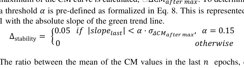
10 ቚ < 𝜀𝜀 · 𝑚𝑚𝑚𝑚𝑚𝑚 𝑔𝑔(𝑥𝑥), 𝜀𝜀 = 0.05 (7) To assess the stability of the CM curve in the last epochs, the standard deviation of the differences between each pair of consecutive points after the maximum of the CM curve is calculated, ΔCM𝑎𝑎𝑎𝑎𝑎𝑎𝑎𝑎𝑎𝑎 𝑚𝑚𝑚𝑚𝑚𝑚. To determine stability, a threshold 𝛼𝛼 is pre-defined as formalized in Eq. 8. This is represented in Figure 1 with the absolute slope of the green trend line.
(8)
Equation reproduced from the original PDF.
0 𝑜𝑜𝑜𝑜ℎ𝑒𝑒𝑒𝑒𝑒𝑒𝑒𝑒𝑒𝑒𝑒𝑒
The ratio between the mean of the CM values in the last 𝑛𝑛 epochs, denoted as 𝜇𝜇𝜇𝜇𝜇𝜇𝜇𝜇𝑎𝑎𝑎𝑎𝑎𝑎 and the maximum CM value evaluates whether the CM has sufficiently decreased over time. A failure to exhibit a meaningful decrement may suggest that both the generator and discriminator are not progressing effectively.
The ideal scenario corresponds to the first case in Eq. 9, where the CM curve demonstrates significant decline, approaching values close to zero by the end of training. Case 2 represents an outcome where there is a notable difference between max𝐶𝐶𝐶𝐶 and the final 𝑛𝑛 values. Finally, case 3 correspond to those cases where there is little to no reduction in CM, indicating insufficient training progress and therefore requiring penalization. Although a valid CM curve may still receive a penalty if its evolution is insufficient, this penalty is less severe than that applied to invalid curves, as minor reductions can often be corrected through small hyperparameter adjustments.
The values of the weights and constants are determined experimentally through multiple training runs across different scenarios to ensure generalization across configurations and datasets. In particular, the negative score of -0.1 assigned to invalid CM curves aims to penalize cases that exhibit poor convergence dynamics.
Quantifying CTGAN Training Dynamics: A Convergence-Aware Self-Adaptive Framework 647
Composite Quality Metric and Final Objective Function To complement the CM score, a Composite Quality Metric (CQM) is used to evaluate the fidelity of the generated data. The CQM combines two components: Column Shapes and Column Pair Trends, capturing both marginal distributions and relationships between variables.
Column Shapes assesses the similarity between real and synthetic marginal distributions. In this study, similarity is evaluated using the Kolmogorov– Smirnov distance for continuous columns and the Total Variation distance for discrete columns.
Column Pair Trends evaluates whether relationships between pairs of columns are preserved. For continuous pairs, similarity is computed using correlation similarity based on Pearson correlations, while for pairs involving discrete variables, contingency similarity compares the joint probability distributions.
The CQM is defined as the arithmetic mean of Column Shapes and Column Pair Trends. Values close to 1 indicate strong similarity between real and synthetic data, reflecting the preservation of both marginal distributions and inter-column relationships. The objective function for hyperparameter optimization is defined as the sum of the CM Score and the CQM.
RESULTS Results on known datasets To evaluate the effectiveness of the proposed algorithm, experiments were first conducted on three publicly available benchmark datasets: the Adult dataset (Becker & Kohavi, 1996), the Chess dataset (Shapiro, 1989), and the Hotel Booking dataset (Antonio et al., 2019). For each test study, 20 execution trials were conducted, with each configuration tested in three separate runs, resulting in a total of 40 evaluations to account for the stochasticity of the training process.
Table 1 presents the hyperparameter importance for each optimization process computed using Optuna’s fANOVA method, revealing that learning rates consistently dominate the optimization process across datasets.
Table 1. Hyperparameter Importance Across Datasets Set D LR G LR B PAC D Dim G Dim 1 0.330 0.429 0.111 0.052 0.039 0.066 2 0.035 0.944 0.000 0.000 0.008 0.008 3 0.057 0.751 0.000 0.000 0.036 0.155 Set: Dataset, D: Discriminator, G: Generator, LR: Learning Rate, B: Batch Size; Dim: Dimensions.
Table 2 reports the best-performing configurations identified for each dataset. For instance, for Dataset 1, the resulting hyperparameters are largely consistent with those reported in the literature (Xu et al., 2019), with the only difference being the learning rates, as the original model employs 2e-4 for both the discriminator and generator. All top-performing configurations achieve positive CM scores, indicating effective convergence during training. In addition, the Overall Score (OS)—computed from the CQM and CM metric—confirms the ability of the model to generate high-quality synthetic data. Table 2. Top-performing configurations and metrics (known datasets)
648 Gregores Coto, Andrea. et al.
In contrast, the worst-performing configurations (Table 3) exhibit negative CM scores, indicating poor convergence during training. Although some configurations still achieve moderate OS due to partial preservation of the statistical properties of data (CQM), the negative CM values reveal unstable generator–discriminator dynamics and therefore unreliable data generation.
Table 3. Bottom-performing configurations (known datasets) Set D LR G LR Batch PAC D Dim G Dim CM OS 1 2.35e-05 1.41e-05 300 20 (256, 256) (512, 512) -0.1 0.917 2 4.04e-05 4.93e-04 140 20 (1024, 512) (512, 512) -0.1 0.622 3 2.40e-04 1.89e-04 140 20 (512, 512) (1024, 512) -0.1 0.538 Set: Dataset, D: Discriminator, G: Generator, LR: Learning Rate, B: Batch Size; Dim: Dimensions, CM: Convergence Metric, OS: Overall Score
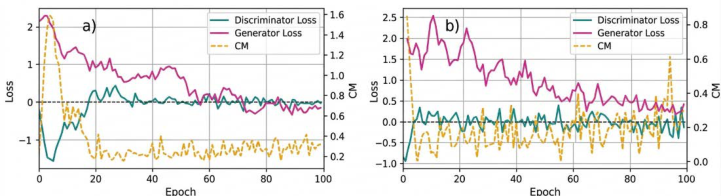
Figure 2 compares the convergence behaviour of the best (a) and worst (b) configurations for Dataset 1 through the loss functions and CM curves. For the best configuration (see Table 2), the CM curve (yellow) increases, reaches an early peak, and subsequently stabilizes, indicating balanced generator– discriminator dynamics. In contrast, the worst configuration (see Table 3) fails to converge, as reflected by unstable loss trajectories and a late upward trend in the CM curve. These results highlight the importance of incorporating an additional metric such as the CM to evaluate convergence alongside synthetic data quality.
Figure 2. Loss and CM curves for the best (a) and worst (b) configurations (Dataset 1).
Results on a real scenario This section evaluates the proposed algorithm using a high-dimensional industrial dataset containing 2,756 rows and 296 features, where each row represents combinations of material properties required for aluminium ingot production. Due to commercial sensitivity, the full dataset cannot be publicly shared; however, an archived dataset with comparable dimensionality and feature heterogeneity is available (Fernández Martínez & Angosto Artigues, 2024), enabling reproduction of the methodological workflow (Fernández Martínez & Gregores, 2026).
Quantifying CTGAN Training Dynamics: A Convergence-Aware Self-Adaptive Framework 649
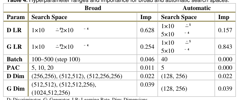
To assess the impact of dataset-driven search space design, two approaches are compared: (1) a broad predefined search space based on prior knowledge, and (2) an automatic search space derived from dataset properties such as sparsity, variance and dimensionality (Fernández Martínez, 2026).
Table 4 compares the hyperparameter ranges explored in the broad and automatic search spaces together with their importance values. The results show that, in the broad search space, the learning rates—particularly the discriminator learning rate—are the most influential parameters in the optimization process. This observation supports the design of the automatic search space, where the remaining parameters are fixed and the optimization focuses solely on the learning rates by design. By concentrating the search on the most relevant parameters, the algorithm reduces unnecessary exploration and improves efficiency, decreasing the number of trials from 25 to 20 while maintaining comparable performance.
Table 4. Hyperparameter ranges and importance for broad and automatic search spaces.
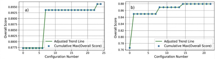
Figure 3 shows the performance evolution across optimization trials for both case studies: a) broad, and b) automatic search space. In general, higher configuration numbers correspond to improved performance. The broad search space requires more trials before improvements appear but stabilizes earlier, whereas the automatic search space achieves faster initial improvements while continuing to evolve more gradually. This behaviour reflects the exploration–exploitation trade-offs between the two approaches.
Figure 3. Performance evolution across trials for (a) broad and (b) automatic search spaces.
650 Gregores Coto, Andrea. et al.
Table 5 reports the best configuration identified for each search strategy together with the corresponding evaluation metrics. Both approaches achieve similar CM and OS values, indicating comparable convergence behaviour and synthetic data quality despite the reduced search space in the automatic strategy.
Table 5. Top-performing configurations and metrics (Real Scenario). Space D LR G LR B PAC D Dim G Dim CM OS B 9.16e-05 1.03e-05 400 10 (512, 512) (512, 512) 0.090 0.895 A 7.03e-05 1.05e-05 40 5 (128, 256) (128, 256) 0.090 0.894 A: Automatic, B: Broad, D: Discriminator, G: Generator, LR: Learning Rate, B: Batch Size; Dim: Dimensions, CM: Convergence Metric, OS: Overall Score.
Table 6 presents the bottom-performing configurations for each search strategy together with their corresponding evaluation metrics. In both cases, the configurations yield negative CM scores, indicating the absence of proper convergence during training.
Table 6. Bottom-performing configurations and metrics (Real Scenario). Search D LR G LR B PAC D Dim G Dim CM OS B 3.08e-05 4.64e-05 400 20 (512, 256) (512, 256) -0.1 0.688 A 2.00e-05 6.41e-05 40 5 (128, 256) (128, 256) -0.1 0.697 A: Automatic, B: Broad, D: Discriminator, G: Generator, LR: Learning Rate, B: Batch Size; Dim: Dimensions, CM: Convergence Metric, OS: Overall Score
A comparison of Tables 5 and 6 shows that CM scores clearly separate well- converged and poorly converged models, supported by the Overall Score (OS) that reflects the combined effect of convergence behaviour and synthetic data quality.
Overall, both search strategies achieve comparable performance. However, the automatically defined search space reduces computational effort, reaching similar results earlier in the process. By focusing on narrower hyperparameter ranges, the algorithm avoids unnecessary exploration and accelerates convergence.
CONCLUSIONS This work proposes a convergence-aware hyperparameter optimization approach for CTGAN training. The method combines a Convergence Metric (CM), which evaluates generator–discriminator training dynamics, with a Composite Quality Metric (CQM) that assesses the fidelity of the generated data. These metrics guide a self-adaptive optimization process that progressively refines the search space.
Results show that the proposed framework enables stable GAN training while maintaining high synthetic data quality. The comparison between broad and automatic search spaces further demonstrates that efficient optimization can be achieved without compromising performance.
The approach is particularly relevant for materials science applications, where datasets are often tabular and experimentally constrained. By enabling reliable data generation and stable model tuning, the approach provides a foundation for future advances in generative modelling and adaptive optimization strategies.
Quantifying CTGAN Training Dynamics: A Convergence-Aware Self-Adaptive Framework 651
ACKNOWLEDGMENT This work has been supported by the project “self-X Artificial Intelligence for European Process Industry digital transformation” (s-X-AIPI), which has received funding from the European Union’s Horizon Europe research and innovation programme under grant agreement No.101058715 and partially by the IRIDISCENTE project (PLEC2023-010190) Artificial intelligence for the sustainable design of efficient alloys and processes (Project PLEC2023-010190), funded under the Transmisiones 2023 programme by the Spanish Ministry of Science and Innovation, through the Agencia Estatal de Investigación (AEI) and CDTI Innovación.
REFERENCES Akiba, T., Sano, S., Yanase, T., Ohta, T., & Koyama, M. (2019). Optuna: A Nextgeneration Hyperparameter Optimization Framework. Proceedings of the ACM SIGKDD International Conference on Knowledge Discovery and Data Mining, 2623–2631. https://doi.org/10.1145/3292500.3330701 Angosto Artigues, R., Fernández Martínez, A., Gregores Coto, A., & Torrez Herrera, J. J.
(2025). A Self-Adaptive ML Pipeline for Sustainable Manufacturing. 437–454. https://doi.org/10.1007/978-981-96-7945-4_27 Antonio, N., de Almeida, A., & Nunes, L. (2019). Hotel booking demand datasets. Data in Brief, 22, 41–49. https://doi.org/10.1016/j.dib.2018.11.126 Arjovsky, M., Chintala, S., & Bottou, L. (2017). Wasserstein Generative Adversarial
Networks (pp. 214–223). PMLR. https://proceedings.mlr.press/v70/arjovsky17a.html Artigues, R. A., Coto, A. G., Herrera, J. J. T., Tomás, F. Lou, Verardi, S., Marzano, M.
G., & Martinez, A. F. (2024). An AI-Driven User-Centric Framework reinforced by Autonomic Computing: A case study in the Aluminium sector. Human Interaction and Emerging Technologies (IHIET 2024), 157(157). https://doi.org/10.54941/ahfe1005478 Becker, B., & Kohavi, R. (1996). Adult - UCI Machine Learning Repository.
https://archive.ics.uci.edu/dataset/2/adult Dumont, V., Ju, X., & Mueller, J. (2022). Hyperparameter Optimization of Generative Adversarial Network Models for High-Energy Physics Simulations. https://doi.org/10.21203/rs.3.rs-2181360/v1 Fernández Martínez, A. (2026). Adaptive Machine Learning Utilities for Data-Aware
Model Tuning. https://doi.org/10.5281/ZENODO.18712765 Fernández Martínez, A., & Angosto Artigues, R. (2024). s-X-AIPI Aluminium DataVault.
https://doi.org/10.5281/ZENODO.10716152 Fernández Martínez, A., & Gregores, A. (2026). s-X-AIPI Aluminium ML Recipe Generator - Convergence Metric and Optimization Framework for CTGAN. https://doi.org/10.5281/ZENODO.18712801 Goodfellow, I., Pouget-Abadie, J., Mirza, M., Xu, B., Warde-Farley, D., Ozair, S.,
Courville, A., & Bengio, Y. (2020). Generative adversarial networks. Communications of the ACM, 63(11), 139–144. https://doi.org/10.1145/3422622 Gulrajani, I., Ahmed, F., Arjovsky, M., Dumoulin, V., & Courville, A. (2017). Improved Training of Wasserstein GANs. Advances in Neural Information Processing Systems, 2017-December, 5768–5778. http://arxiv.org/abs/1704.00028 Lin, Z., Khetan, A., Fanti, G., & Oh, S. (2018). PacGAN: The power of two samples in
generative adversarial networks. IEEE Journal on Selected Areas in Information Theory, 1(1), 324–335. http://arxiv.org/abs/1712.04086 Saxena, D., & Cao, J. (2022a). Generative Adversarial Networks (GANs). ACM Computing Surveys, 54(3), 63. https://doi.org/10.1145/3446374 Saxena, D., & Cao, J. (2022b). Generative Adversarial Networks (GANs). ACM
652 Gregores Coto, Andrea. et al.
Computing Surveys, 54(3), 63. https://doi.org/10.1145/3446374 Shapiro, A. (1989). Chess (King-Rook vs. King-Pawn) - UCI Machine Learning Repository. https://archive.ics.uci.edu/dataset/22/chess+king+rook+vs+king+pawn Watanabe, S. (2025). Tree-Structured Parzen Estimator: Understanding Its Algorithm
Components and Their Roles for Better Empirical Performance. http://arxiv.org/abs/2304.11127 Xu, L., Skoularidou, M., Cuesta-Infante, A., & Veeramachaneni, K. (2019). Modeling Tabular data using Conditional GAN. Advances in Neural Information Processing Systems, 32. https://github.com/DAI-Lab/CTGAN
LISTED IN THE AHFE DIGITAL BOOKSTORE CATALOGUE
Explore the complete digital volume
Human Interaction and Emerging Technologies (IHIET-AI 2026): Artificial Intelligence and Future Applications
Read this individual research paper free through the original publisher, or explore the full digital proceedings book.
ISBN 978-1-964867-77-9
Explore this ISBN in the AHFE Bookstore ↗Listed in the July 2026 bookstore catalogue; search by ISBN to confirm current availability · Digital book purchase optional